EECE 340 Chapter 11, Fall 2011

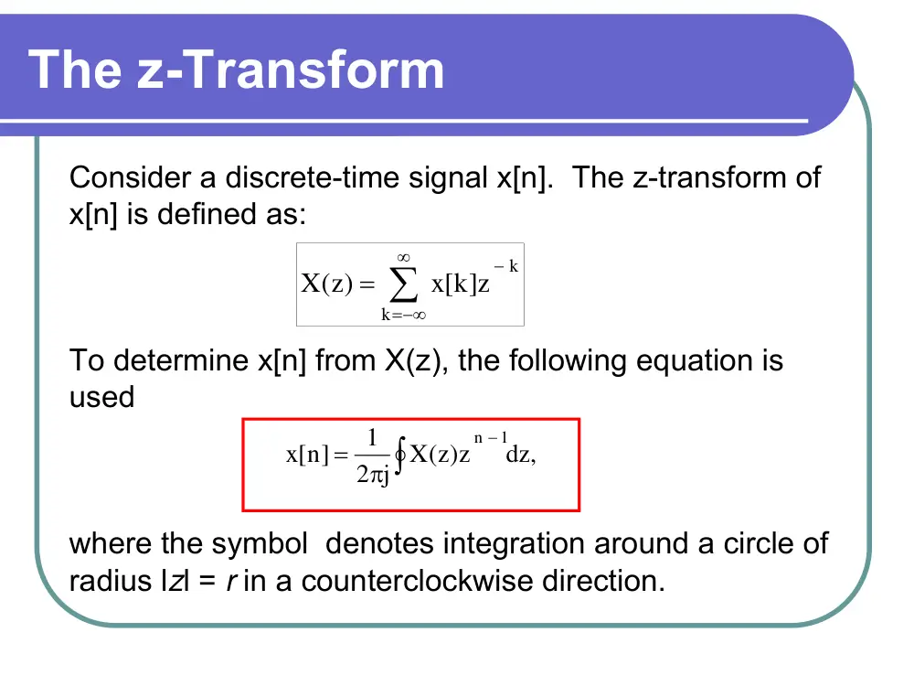
Chapter 11 The Z-transform Introduction � The z-transform is considered to be the discrete-time counterpart to the Laplace transform. � With the use of the z-transform, we will be able to obtain a broader characterization of discrete-time LTI systems and their interaction with signals. The z-Transform Consider a discrete-time signal x[n]. The z-transform of x[n] is defined as: To determine x[n] from X(z), the following equation is used where the symbol denotes integration around a circle of radius lzl = r in a counterclockwise direction. 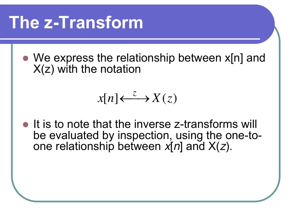∑ ∞ −∞ = − = k k x[k z] (z) X dz, 2 j X( )z z 1 x[n] n 1 ∫ − π = The z-Transform � We express the relationship between x[n] and X(z) with the notation � It is to note that the inverse z-transforms will be evaluated by inspection, using the one-to- one relationship between x[n] and X(z). ( ) [ ] X z x n z ⎯→ ← Convergence � The z-transform exists when the infinite sum in the definition converges. A necessary condition for the convergence is absolute summability of x[n]z-n Since |x[n]z-n| = |x[n]r-n|, we must have � The range of r for which this condition is satisfied is termed the region of convergence (ROC) of the z-transform. 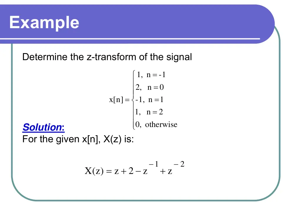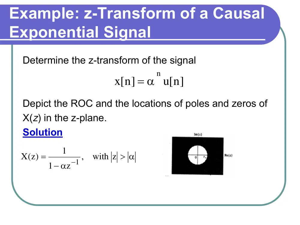< ∞ ∑ ∞ −∞ = x[n r] − | | n n Example Determine the z-transform of the signal Solution: For the given x[n], X(z) is: ⎪ ⎪ ⎪ ⎩ ⎪⎪ ⎪ ⎨ ⎧ = = = = = otherwise 0, n 2 1, -1, n 1 n 0 2, 1, n - 1 [n] x 2 1 z z 2 z X(z) − − + − + = Example: z-Transform of a Causal Exponential Signal Determine the z-transform of the signal Depict the ROC and the locations of poles and zeros of X(z) in the z-plane. 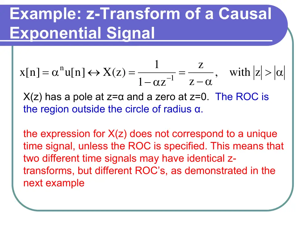Solution u[n] x[n] α n = > α − α = − , with z z 1 1 X(z) 1 Example: z-Transform of a Causal Exponential Signal X(z) has a pole at z=α and a zero at z=0. The ROC is the region outside the circle of radius α. the expression for X(z) does not correspond to a unique time signal, unless the ROC is specified. 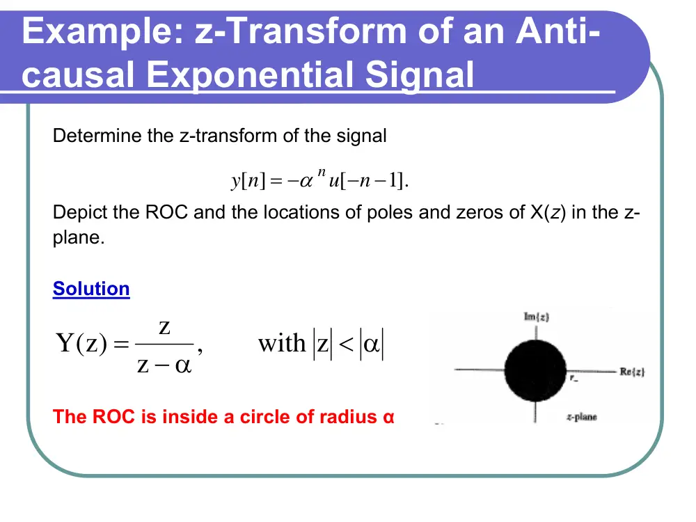This means that two different time signals may have identical z- transforms, but different ROC’s, as demonstrated in the next example > α − α = − α = ↔ = α − , with z z z z 1 1 X(z) u[n] x[n] 1 n Example: z-Transform of an Anti- causal Exponential Signal Determine the z-transform of the signal Depict the ROC and the locations of poles and zeros of X(z) in the z- plane. Solution The ROC is inside a circle of radius α < α − α = , with z z z (z) Y 1]. [ [ ] − − = − n u y n α n To conclude � Note that Y(z) in the last two examples are the same, except for the region of convergence, even though the time signals are quite different. Only the ROC differentiates the two transforms. � We must know the ROC to determine the correct inverse z-transform. � This ambiguity is a general feature of signals that are one sided. Example: z-transform of A Two- Sided Signal Determine the z-transform of Depict the ROC and the locations of poles and zeros of X(z) in the z- plane. Solution: The ROC is the plane between the 2 circles. 1 z 2 , with 1 )1 (z z ( (z 2z X( )z 2 ) 1 2 ) 3 < < − − − = u[n]. 2 1 ]1 u[ n x[n] n ⎟ ⎠ ⎞ ⎜ ⎝ + ⎛ − − = − Problems Determine the z-transform and the ROC for the following signals 2 1 with z ), )(z z ( ) z(2z X(z) u[n] 3 1 u[n] 2 1 [n] x 3 1 2 1 6 1 n n > + − − = ↔ ⎟ ⎠ ⎞ ⎜ ⎝ + ⎛ − ⎟ ⎠ ⎞ ⎜ ⎝ ⎛ = 3 1 with z ), )(z z ( ) z(2z X( )z ]1 u[ n 3 1 ]1 u[ n 2 1 [n] x 3 1 2 1 6 1 n n < + − − = ↔ − − ⎟ ⎠ ⎞ ⎜ ⎝ −⎛ − − − ⎟ ⎠ ⎞ ⎜ ⎝ = −⎛ Problems 4 3 3 1/3), with 1 3/ 4)( ( 5/12) (2 ( ) [ ] 3 1 ]1 [ 4 3 [ ] < < + − − = ↔ ⎟ ⎠ ⎞ ⎜ ⎝ + ⎛ − − − ⎟ ⎠ ⎞ ⎜ ⎝ = −⎛ z z z z z X z u n n u n x n n Properties of the Z-transform 1. Linearity x z tranform X(z) with ROC R x[n] ⎯ ⎯⎯⎯⎯ → ← − y z tranform Y(z) with ROC R [y n] ⎯ ⎯⎯⎯ → ← − y x z tranform R bY(z) with ROC R aX(z) by[n] ax[n] ∩ + ⎯ ⎯⎯⎯⎯ → ← + − Example Suppose Determine the z-transform of ax[n]+by[n] 2 3 z 2 ROC 1 with 2 3 z 2 1 z z X( )z ]1 u[ n 2 3 u[n] 2 1 [n] x n n < < ⎟⎠ ⎞ ⎜⎝ ⎛ − ⎟⎠ ⎞ ⎜⎝ ⎛ − − = ↔ − − ⎟ ⎠ ⎞ ⎜ ⎝ −⎛ ⎟ ⎠ ⎞ ⎜ ⎝ ⎛ = 1 2 ROC z with 2 1 z 4 1 z 4 z 1 Y( )z u[n] 2 1 u[n] 4 1 n] [y n n > ⎟⎠ ⎞ ⎜⎝ ⎛ − ⎟⎠ ⎞ ⎜⎝ ⎛ − − = ↔ ⎟ ⎠ ⎞ ⎜ ⎝ −⎛ ⎟ ⎠ ⎞ ⎜ ⎝ ⎛ = 2 3 z 2 1 with ROC 1 z 1 z 4 z b 3 z 1 z z a by[n] ax[n] z tan sfrom < < ⎟⎞ ⎟⎞⎜⎛ − ⎜⎛ − 2 4 2 2 ⎠ ⎝⎠ ⎝ − + ⎟⎞ ⎟⎞⎜⎛ − ⎜⎛ − − ⎯ ⎯⎯⎯⎯ → ← + − ⎠ ⎝⎠ ⎝ 2. Time Reversal Let Then, x z tranform X(z) with ROC R x[n] ⎯ ⎯⎯⎯⎯ → ← − x z transform R z , with ROC 1 X 1 x[ n] ⎟ ⎠ ⎞ ⎜ ⎝ ⎛ ⎯ ⎯⎯⎯⎯ → ← − − 3. Time shifting Let Then, x z tranform X(z) with ROC R x[n] ⎯ ⎯⎯⎯⎯ → ← − = ∞ = ⎯ ⎯⎯⎯ → ← − − − 0 or z except possibly z , X(z) with ROC R z n ] x[n x n0 z transform 0 4. Multiplication by an exponential sequence Let Then, x z tranform X(z) with ROC R x[n] ⎯ ⎯⎯⎯⎯ → ← − x z transform n R X z with ROC x[n] α ⎟ ⎠ ⎞ ⎜ ⎝ ⎛ α ⎯ ⎯⎯⎯⎯ → ← α − 5. Convolution Let Then, x z tranform X(z) with ROC R x[n] ⎯ ⎯⎯⎯⎯ → ← − y z tranform Y( )z with ROC R [y n] ⎯ ⎯⎯⎯ → ← − y x z transform R X(z)Y(Z) with ROC at least R x[n]* [y n] ∩ ⎯ ⎯⎯⎯⎯ → ← − 6. Differentiation in the z-domain Let Then, x z tranform X(z) with ROC R x[n] ⎯ ⎯⎯⎯⎯ → ← − x z transform dz X(z) with ROC R z d nx[n] − ⎯ ⎯⎯⎯⎯ → ← − Example: Applying Multiple Properties Find the z-transform of Solution ⎟ ⎟ ⎠ ⎞ ⎜ ⎜ ⎝ ⎛ − ⎟ ⎠ ⎞ ⎜ ⎝ ⎟∗ ⎛ ⎟ ⎠ ⎞ ⎜ ⎜ ⎝ ⎛ ⎟ ⎠ ⎞ ⎜ ⎝ ⎛ − = − u[ n] 4 1 u[n] 2 1 n x[n] n n 2 1 with ROC z , 2 1 z z u[n] 2 1 z n > + ⎯→ ← ⎟ ⎠ ⎞ ⎜ ⎝ ⎛ − 2 1 ROC z with 2 1 z 2 z 1 2 1 z z dz z d u[n] 2 1 n 2 z n > ⎟⎠ ⎞ ⎜⎝ ⎛ + − = ⎟⎟ ⎟ ⎟ ⎠ ⎞ ⎜⎜ ⎜ ⎜ ⎝ ⎛ + ⎯→− ← ⎟ ⎠ ⎞ ⎜ ⎝ ⎛ − Example: Cont’d 4 1 with ROC z , 4 1 z z u[n] 4 1 z n > − ⎯→ ← ⎟ ⎠ ⎞ ⎜ ⎝ ⎛ 4 z - 4 , with ROC z - 4 4 1 z 1 z 1 u[ n] 4 1 z n < = − ⎯→ ← − ⎟ ⎠ ⎞ ⎜ ⎝ ⎛ − ( ) 4 z 2 with ROC 1 , 2 1 4 z z 2z x[n] 2 z < < ⎟ ⎠ ⎞ ⎜ ⎝ ⎛ + − ⎯→ ← Inversion of the z-transform Partial-Fraction Expansion In most cases, the z-transform may be written as and assume that M<N. If M>N, the we may use long division. The partial-fraction expansion of X(z) is obtaining by factoring the denominator of X(z) into a product of first-order terms. That is Depending on the ROC and the order of the pole, the inverse z- transform associated with each term in then determined by using the appropriate transform pair N N 2 2 1 1 0 M M 2 2 1 1 0 2 1 z a ... a z a z a z ....b b z b z b P (z) P (z) X(z) − − − − − − + + + + + + + = = ∏ = − − − − − + + + = = N 1 k 1 k 0 M M 2 2 1 1 0 2 1 ) d z 1( a z ....b b z b z b P (z) P (z) X(z) Inversion of the z-transform Partial-Fraction Expansion Equations to remember k 1 k k z n k k d with ROC z d z 1 A A (d ) u[n] > − ⎯→ ← − k 1 k k z n k k d with ROC z d z 1 A ]1 A (d ) u[ n < − ⎯→ ← − − − − k 1 m k k z n k k d with ROC z ) d z 1( A (d ) u[n] 1)! (m )1 m 1)...(n (n A > − ⎯→ ← − − + + − k m 1 k k z n k k d with ROC z ) d z 1( A ]1 (d ) u[ n 1)! (m )1 m 1)...(n (n A < − ⎯→ ← − − − − + + − − Example Find the inverse z-transform of Solution ( )( ) 2 z with ROC 1 z 1 2z 1 2 z 1 1 z z 1 X(z) 1 1 1 2 1 < < − ⎟ − ⎠ ⎞ ⎜ ⎝ ⎛ − + − = − − − − − ( ) ( ) z 1 2 2z 1 2 2 z 1 1 1 X( )z 1 1 1 − − − − − − + ⎟ ⎠ ⎞ ⎜ ⎝ ⎛ − = ( ) ]1 2(2) u[ n u[n] 2 1 u[n] 2 1 x[n] n n n − − − − ⎟ ⎠ ⎞ ⎜ ⎝ = ⎛ Example: Inversion of an improper rational function Find the inverse z-transform of Solution where 1 with ROC z 4 2z z 2 4 4z 10z z X(z) 2 2 3 < − − + − − = 2 zW(z); 1 X(z) = 1 with ROC z 2z 1 3 z 1 1 3 2z W(z) 1 1 1 < − − + + + = − − − − ]1 2 w[n 1 x[n] + = ( ) ]1 3(2) u[ n ]1 u[ n 1 3 [n] ]1 2 [n w[n] n n − − + − − − − + δ − = − δ Example: Inversion using Power series expansion Find the inverse z-transform of using a power series expansion Solution We use long division to write X(z) as a power series in z-1 since the ROC indicates that x[n] is right sided. We have 2 1 with ROC z 2 z 1 1 z 2 X(z) 1 1 > − + = − − ....... 5.0 z z 2z 2 X(z) 3 2 1 + + + + = − − − ...... 3] [n 5.0 2] [n ]1 2 [n 2 [n] x[n] + − δ + − + δ − + δ = δ The Transfer Function Consider a LTI discrete-time system whose input is x[n] and output y[n]. The output can be expressed as the convolution of the impulse response h[n] and the input x[n] y[n] = x[n] * h[n] If we take the z-transform of both sides of the equation, we will obtain Y(z)=H(z)X(z) H(z) is called the system transfer function which is defined as the ratio of the z-transforms of the output to that of the input X(z) Y(z) H(z) = The Transfer Function X(z) Y(z) H(z) = In order to determine the impulse response of the system (inverse z-transform), the ROC must be given. If ROC is not known, then other system characteristics, such as stability or causality, must be known in order to uniquely determine the impulse response. Example: System Identification The problem of finding the system description from knowledge of the input and output is known as system identification. Find the transfer function and impulse response of a causal LTI system if the input to the system is and Solution: The z-transforms of the input and output are respectively given by: ( ) u[n] 1/3 x[n] n − = ( ) u[n] 1/3 u[n] )1 (3 [y n] n n + − = ( ) 3 1 with ROC z /3 z 1 1 X(z) 1 > + = − Example: System Identification The transfer function of the system is: Impulse response: The impulse response is thus given by: 1 with ROC z 1( /3)z 1 1 z 1 3 Y(z) 1 1 > − + + = − − 1 with ROC z 1( /3)z ) z )(1 1( ) 1( /3)z 4 1( H(z) 1 1 1 > − + + = − − − 1 with ROC z 1( /3)z ) 1( 2 z ) 1( 2 H(z) 1 1 > − + + = − − [ ] 2 1( /3) [ ] )1 2( [ ] u n u n h n n n + − = Example: The transfer function of an LTI system described by a difference equation Determine the transfer function and the impulse response for the causal LTI system described by the difference equation. Solution Using the z-transform, we obtain: The system is causal, so we choose the right-sided inverse z- transform for each term to obtain the following impulse response: ]1 2x[n x[n] 2] 8 [y n 3 ]1 4 [y n 1 [y n] − + = − − − − − 1 1 2 1 1 1 (3/ 4) 1 1( / 2) 1 2 (3/8) 1( / 4) 1 2 1 ) ( − − − − − + − + − = − − − + = z z z z z z H u[n] 4 3 u[n] 2 1 2 [n] h n n ⎟⎠ ⎞ ⎜⎝ + ⎛ ⎟⎠ ⎞ ⎜⎝ = − ⎛− Example: Finding A Difference- Equation Description Find the difference- equation description of an LTI system with transfer function Solution This system is described by the difference equation y[n] + 3y[n - 1] + 2y[n - 2] = 5x[n - 1] + 2x[n - 2]. 2 3z z 2 5z H(z) 2 + + + = Causality and Stability � The impulse response of a causal LTI system is zero for n<0. Therefore, the impulse response of a causal LTI system is determined from the transfer function by using right-sided inverse transforms. A pole that is inside the unit circle in the z-plane contributes an exponentially decaying term to the impulse response, while a pole that is outside the unit circle contributes an exponentially increasing term. � Therefore, - A system is stable if the ROC includes the unit circle - A system is stable and causal if all poles of the transfer function are inside the unit circle. Example: Causality and stability An LTI system has the transfer function Find the impulse response, assuming that the system is stable Solution: The given system has poles at z=-2, and If the system is stable, then the ROC includes the unit circle. The two poles inside the unit circle contribute right-sided terms to the impulse response, while the pole outside the unit circle contributes a left-sided term. Hence, 1 1 j4 1 j4 2z 1 3 z 9.0 e 1 2 z 9.0 e 1 2 H(z) − − − π − π + + − + − = j4 9.0 e z π = j4 9.0 e z − π = ]1 3( 2) u[ n u[n] 9.0 e 2 u[n] 9.0 e 2 h[n] n n j 4 n j4 − − − − ⎟⎟ ⎟ ⎠ ⎞ ⎜⎜ ⎜ ⎝ ⎛ + ⎟⎟ ⎟ ⎠ ⎞ ⎜⎜ ⎜ ⎝ ⎛ = − π π Example: Causality and stability An LTI system has the transfer function Find the impulse response, assuming that the system is causal. Solution: The given system has poles at z=-2, and If the system is assumed causal, then all poles contribute right-sided terms to the impulse response, we have 1 1 j4 1 j4 2z 1 3 z 9.0 e 1 2 z 9.0 e 1 2 H(z) − − − π − π + + − + − = j4 9.0 e z π = j4 9.0 e z − π = 3( 2) u[n] u[n] 9.0 e 2 u[n] 9.0 e 2 h[n] n n j4 n j4 − + ⎟⎟ ⎟ ⎠ ⎞ ⎜⎜ ⎜ ⎝ ⎛ + ⎟⎟ ⎟ ⎠ ⎞ ⎜⎜ ⎜ ⎝ ⎛ = − π π Implementing Discrete-Time LTI Systems; Direct Form I Example: Consider an LTI system described by the difference equation Taking the z-transform of this difference equation gives 2] b x[n ]1 b x[n b x[n] 2] [y n a ]1 [y n a [y n] 2 1 0 2 1 − + − + = − + − + 2 2 1 1 2 2 1 1 0 a z a z 1 b z b z b X(z) Y(z) H(z) − − − − + + + + = = Implementing Discrete-Time LTI Systems; Direct Form II Direct Form II was obtained by simply interchanging the order of the two systems EXAMPLE Consider a system represented by the transfer function Depict the cascade form for this system, using real-valued second-order sections. Assume that each second-order section is implemented as a direct form II representation. Solution: We combine complex-conjugate poles and zeros into the sections, obtaining ( )( ) ) z .0 75e )(1 z .0 75e 1( z 5.0 e 1 z 5.0 e 1 ) z )(1 jz )(1 jz 1( H(z) 1 j / 8 1 j / 8 1 j / 4 1 / 4 j 1 1 1 − π − π − − π − π − − − − − − − + − + = ( 2 ) 1 2 1 .0 25z cos( /4)z 1 z ) 1( H ( )z − − − + π − + = ( 2 ) 1 1 2 (9/16)z cos( /8 z) 5.1 1 ) z 1( H ( )z − − − + π − + = Example Example Depict the parallel-form representation of the transfer function Using first-order sections implemented as a direct form II representation. Answer: ) .0 25z )(1 5.0 z )(1 5.0 z 1( 5.0 z 5.0 z 4 H(z) 1 1 1 2 1 − − − − − − + − − − = ) .0 25z 1( 2 ) 5.0 z 1( 1 ) 5.0 z 1( 1 H(z) 1 1 1 − − − − + + + − = Example Bilinear transformation � The bilinear transformation does a mapping from the s- plane to the z-plane. It maps the jω axis to the unit circle, the left-side of the complex plane to the inside of the unit circle, and the right-side of the complex plane into the outside of the unit circle. The mapping is done by substituting the following into the analog transfer function. � where α is a scaling parameter introduced for flexibility. In the absence of other requirements, it is often set to 1. ⎟⎠ ⎞ ⎜⎝ ⎛ + − = + − = α 1 z 1 z T 2 )1 (z )1 (z s Example: First-order analog filter Consider the analog filter described by: Applying the Bilinear Transformation with α=1, we obtain The resulting digital filter has one simple pole at which is located inside the unit circle. 0 b , b s 1 H )s( > + = 1 1 b z 1 b 1 1 z 1 b 1 1 H( )z − − + − − + ⋅ + = b 1 b 1 z + − =