EECE 340 Chapter 2, Fall 2011

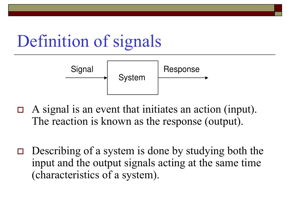
Chapter 2 Continuous-Time Signals and Systems Chapter Outlines � In this chapter, we will be studying some concepts of signals and systems representations in continuous time domain Definition of signals Signal Response System � A signal is an event that initiates an action (input). The reaction is known as the response (output). � Describing of a system is done by studying both the input and the output signals acting at the same time (characteristics of a system). Continuous-Time signals � A signal may be either a Continuous-time signal or a discrete-time signal. � A signal x(t) is said to be a continuous time signal, if it is defined for all values of time t. Discrete-Time signals � A discrete-time signal x(nTs) is a signal that is only define at discrete instants of time. A discrete-time signal is usually derived from a continuous time signal through sampling. Ts is called the sampling period. Therefore, sampling the signal x(t) at time yields a discrete-time signal x(nTs). 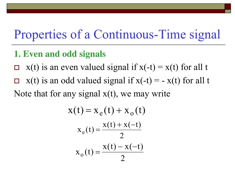For convenience of presentation, we use X[n] = x(n) for n = 0, ± 1, ±2, ±3, …… Properties of a Continuous-Time signal 1. 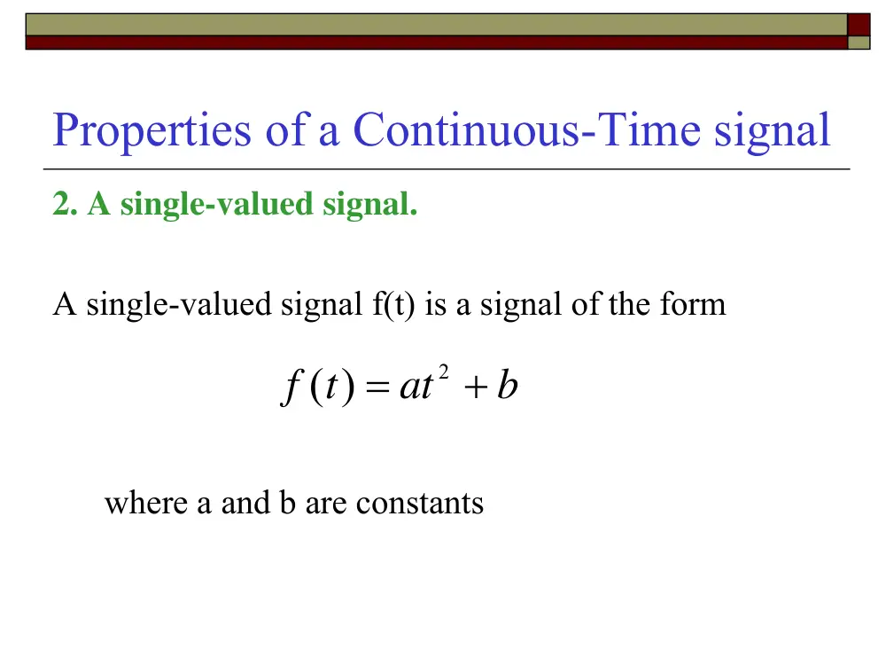Even and odd signals � x(t) is an even valued signal if x(-t) = x(t) for all t � x(t) is an odd valued signal if x(-t) = - x(t) for all t Note that for any signal x(t), we may write )t( x )t( x )t( x o e + = 2 )t x( x )t( )t( xe − + = 2 )t x( x )t( )t( xo − − = Properties of a Continuous-Time signal 2. A single-valued signal. 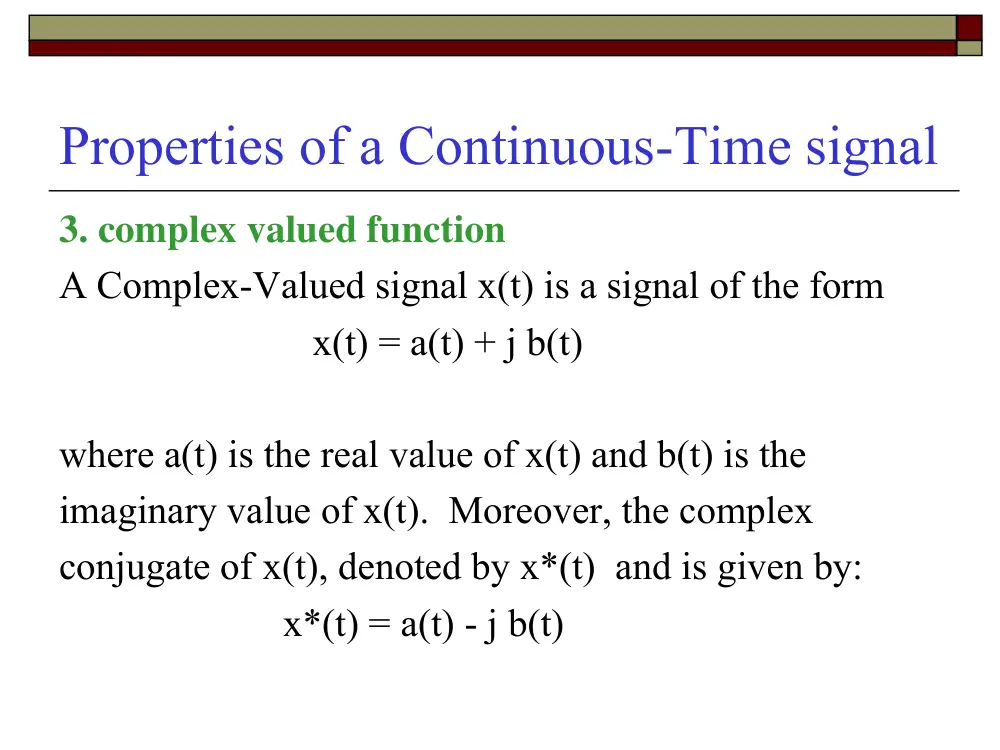A single-valued signal f(t) is a signal of the form where a and b are constants f t at b ( ) = + 2 Properties of a Continuous-Time signal 3. complex valued function A Complex-Valued signal x(t) is a signal of the form x(t) = a(t) + j b(t) where a(t) is the real value of x(t) and b(t) is the imaginary value of x(t). 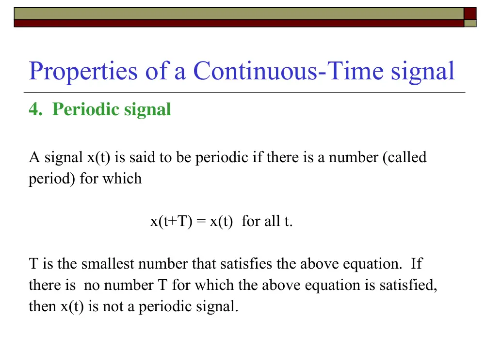Moreover, the complex conjugate of x(t), denoted by x*(t) and is given by: x*(t) = a(t) - j b(t) Properties of a Continuous-Time signal 4. Periodic signal A signal x(t) is said to be periodic if there is a number (called period) for which x(t+T) = x(t) for all t. T is the smallest number that satisfies the above equation. If there is no number T for which the above equation is satisfied, then x(t) is not a periodic signal. Properties of a Continuous-Time signal Examples on periodicity: � x(t)=cost is periodic with a period T=2π. � x(t)=sint+cos√2 t is not periodic � If x(t)=cos(at)+sin(bt). What is the relation between a and b for which x(t) is a periodic function? What will be then the period of x(t)? Properties of a Continuous-Time signal 5. Random signal, Deterministic signal. � A random signal is one about which there is some degree of uncertainty before it actually occurs. Example: The output of an experiment. � A non-random or deterministic signal is one about which there is no uncertainty in its value. Example: x(t)=Acos(ωt+θ) Properties of a Continuous-Time signal 6. A sinusoidal signal: A sinusoidal signal is a signal of the form x(t)=A cos(ωt+θ). This signal plays a very important role in the analysis of communication systems. Notation A is called the amplitude (V or A) ω is called the frequency (rad/s), ω=2πf (Hz) θ is called the phase (rad) Note The principle of Fourier methods of signal analysis is to break up the periodic signals into summations of sinusoidal components. This provides a description of a given signal in terms of sinusoidal frequencies. So if we have to talk about power and energy of a signal, we know how they are distributed along their frequencies. Classification of signals All signals are classified into 3 types 1. Energy Signals 2. Power Signals 3. Neither 1. Energy signals � An energy signal is a pulse-like signal. It exists for only a finite interval of time or, even if present for an infinite amount of time at least has a major portion of its energy concentrated in a finite time interval. Rectangular Pulse Gaussian Pulse t t f t( ) f t e t ( ) = − 2 1. Energy signals For a 1 Ohm resistance, the energy dissipated by the signal during a time interval (t1, t2) is: An energy signal is a signal for which: .dt Joules x )t( E 2 1 t t 2 ∫ = < ∞ ∫ ∞ −∞ .dt )t( x 2 2. Power Signals the instantaneous power dissipated by a voltage v(t) in a resistance R is If the signal is a current signal i(t), then the instantaneous power dissipated in R is: watts R v )t( P 2 = .R watts )t(i P 2 = 2. Power Signals For 1 Ω resistor, the average power dissipated by the signal f(t) during the time interval (t1, t2) is: If and finite when the interval becomes infinite, then f(t) has a finite average power and is called power signal. ∫ − = 2 1 t t 2 1 2 .dt )t( f t t 1 P 0 .dt )t( f T 1 lim / 2 T /2 T 2 T > ∫ − →∞ Classification of Systems A system is usually represented by a box with input and output functions The following notations are mostly used -- g(t)=F{f(t)} -- f(t) →g(t) System f t( ) g t( ) Properties of Systems 1. Linear and Nonlinear Systems A system is linear then superposition applies that is if f1(t) → g1(t) f2(t) → g2(t) then, a f1(t) +b f2(t) → a g1(t) + b g2(t) If the above equation does not apply, then the system is said to be a nonlinear system. Properties of Systems 1. Linear and Nonlinear Systems Examples: a. g(t) = a x(t) b. g(t) = a x(t) + b c. g(t) = a sin [x(t)] Properties of Systems 2.Time-invariant or Time-varying systems � A system is time-invariant if a time shift in the input results in a corresponding time shift in the output 0 0 0 t t )] t( F f[ t ) g t( ∀ − = − Properties of Systems 3. Physically Realizable (Causal) systems � A physically realizable (causal) system can not have an output response before an arbitrary input function is applied. 0 t for 0 g )t( ≤ = Properties of Systems 4. Stable system � A system with input x(t) and output y(t) is said to be stable if the output is bounded for every bounded input. That is, if |x(t)|<M<∞, then |y(t)|<N<∞. Singularity Functions � There is a particular class of functions which plays an important role in signal analysis. Members of this class have simple mathematical forms but they are either not finite everywhere or they do not have finite derivatives of all orders everywhere. For this reason, they are called singularity functions. These functions do not occur in physical systems, but they are useful in signal analysis for good approximation and difficult representations Dirac, delta, or impulse function δ(t) � The most important is the unit impulse response (Dirac, delta) δ(t). This function has the property exhibited by the following integral equation for any continuous f(t0) at t=to ; t0 finite ⎪⎩ ⎪⎨ ⎧ < < = δ − ∫ elsewhere 0 b t a ) f t( t ) dt t( )t( f 0 0 b a 0 Dirac, delta, or impulse function δ(t) Examples 1 log10 10)dt t( t log 0 (x)dx e e )dt e t( e 100 1 1 x 1 cos t cos 2 = = − δ = δ = = − π δ ∫ ∫ ∫ ∞ − − π ∞ −∞ Properties of δ(t) 1. General equation When a and b go to infinity in Then, ⎪⎩ ⎪⎨ ⎧ < < = δ − ∫ elsewhere 0 b t a ) f t( t ) dt t( )t( f 0 0 b a 0 ) f t( t ) dt t( )t( f 0 0 = δ − ∫ ∞ −∞ Properties of δ(t) 2. Area If f(t)=1, then That is δ(t) has a unit area ) f t( t ) dt t( )t( f 0 0 = δ − ∫ ∞ ∞ − − 0 =1 δ∫ +∞ ∞ − t ) t( Properties of δ(t) 3. Amplitude The amplitude at the point t=t0 is undefined. 0 0 t t 0 t ) t( ∀ ≠ = − δ Properties of δ(t) 4. Symmetry 5. Time scaling )t( )t ( = δ − δ )t( a 1 (at) δ = δ Properties of δ(t) 6. Multiplication by a time function It is assumed that f(t) is continuous at t=t0. t ) t( ) f t( t ) t( f t( ) 0 0 0 − δ = − δ The unit step function u(t) The unit step function is that function defined by: ⎪⎩ ⎪⎨ ⎧ < > = − 0 0 0 t t 0 t t 1 t ) t( u t0 t u t t ( ) − 0 Relationship between δ(t) and u(t) If a=-∞, b=t, and f(t)=1, then ⎪⎩ ⎪⎨ ⎧ < < = δ − ∫ elsewhere 0 b t a ) f t( t )dt t( )t( f 0 0 b a 0 t ) t( t ) dt u t( d d) t ( dt d : Or t )dt t( t ) t( u t ) u t( t t t t t )dt t( t t t 0 0 0 0 0 0 0 0 0 0 1 − = δ − τ = τ − δ − δ = − − = ⎪⎩ ⎪⎨ ⎧ ⎪⎭ ⎪⎬ ⎫ < > = − δ ∫ ∫ ∫ ∞ − ∞ − −∞ Relationship between δ(t) and u(t) t0 t u t t ( ) − 0 t t0 d dt u t t t t ( ) ( ) − = − 0 0 δ Example Compute and graph the derivative of the rectangular pulse shown below t0 t f t( ) A Example t ) t( A t( ) A dt t( ) df t ) Au t( Au t( ) t( ) f 0 0 − δ − δ = − − = t0 t f t( ) A f t \( ) A −A t t0