EECE 340 Chapter 13, Fall 2011

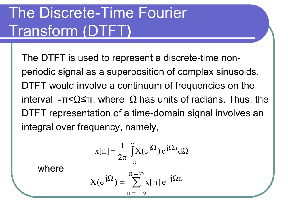
Chapter 13 The Discrete-Time Fourier Transform (DTFT) The Discrete-Time Fourier Transform (DTFT) The DTFT is used to represent a discrete-time non- periodic signal as a superposition of complex sinusoids. DTFT would involve a continuum of frequencies on the interval -π<Ω≤π, where Ω has units of radians. 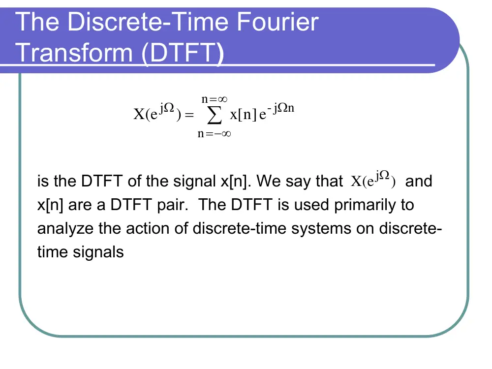Thus, the DTFT representation of a time-domain signal involves an integral over frequency, namely, where ∫ π π − Ω Ω Ω π = d e ) X e( 2 1 x[n] j n j ∑ ∞ = −∞ = Ω Ω = n n n j- j x[n e ] ) X e( The Discrete-Time Fourier Transform (DTFT) is the DTFT of the signal x[n]. We say that and x[n] are a DTFT pair. 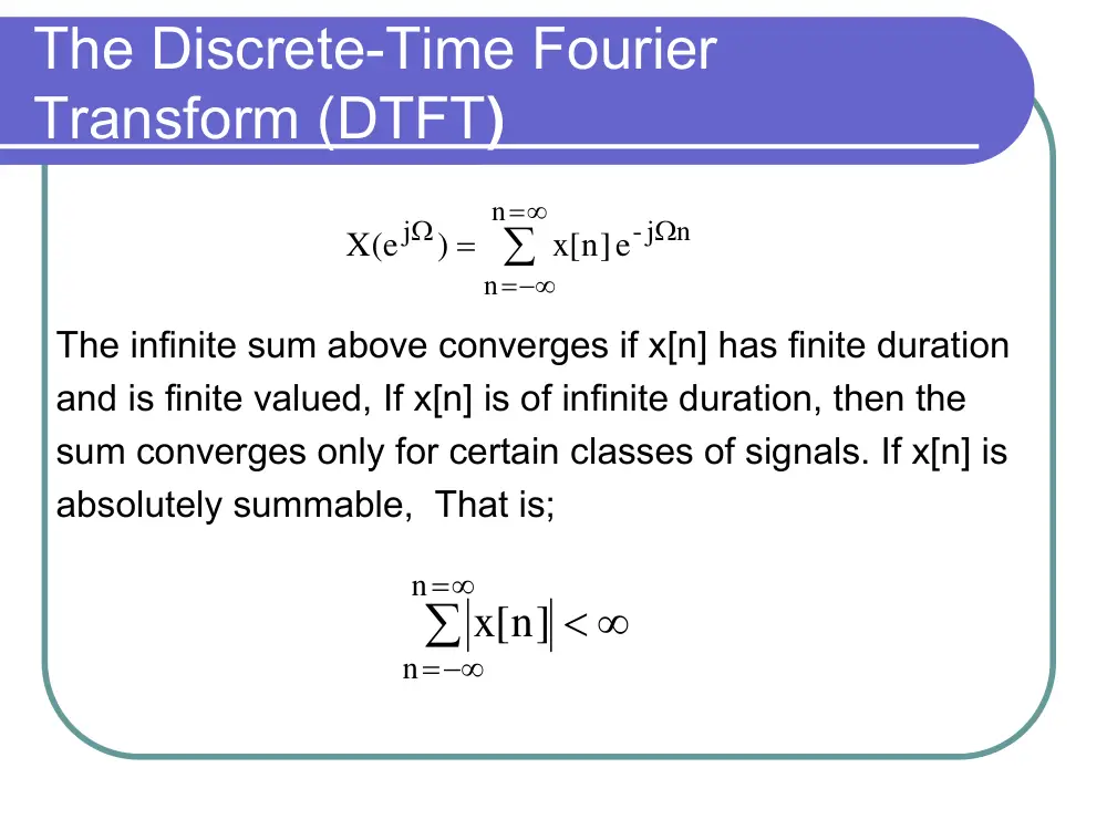The DTFT is used primarily to analyze the action of discrete-time systems on discrete- time signals ∑ ∞ = −∞ = Ω Ω = n n n j- j x[n e ] ) e( X ) X e( jΩ The Discrete-Time Fourier Transform (DTFT) ∑ ∞ = −∞ = Ω Ω = n n n j- j x[n e ] ) e( X The infinite sum above converges if x[n] has finite duration and is finite valued, If x[n] is of infinite duration, then the sum converges only for certain classes of signals. 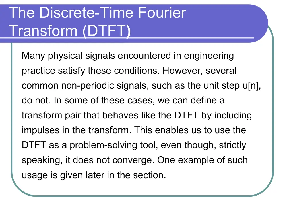If x[n] is absolutely summable, That is; < ∞ ∑ ∞ = −∞ = n n x[n] The Discrete-Time Fourier Transform (DTFT) Many physical signals encountered in engineering practice satisfy these conditions. However, several common non-periodic signals, such as the unit step u[n], do not. In some of these cases, we can define a transform pair that behaves like the DTFT by including impulses in the transform. This enables us to use the DTFT as a problem-solving tool, even though, strictly speaking, it does not converge. One example of such usage is given later in the section. 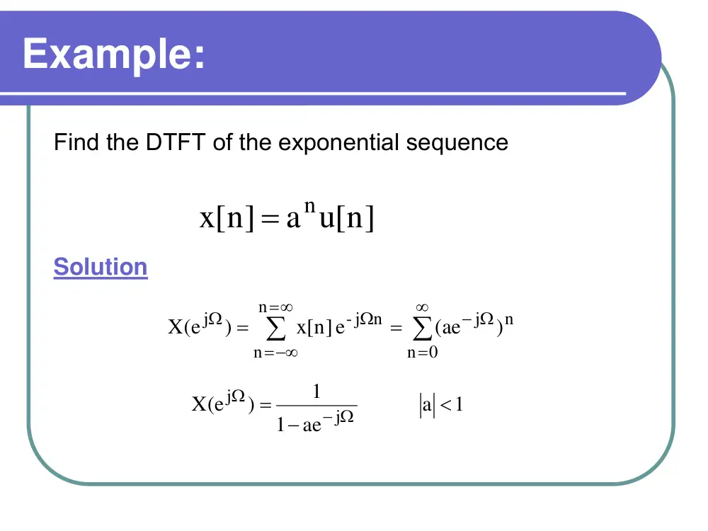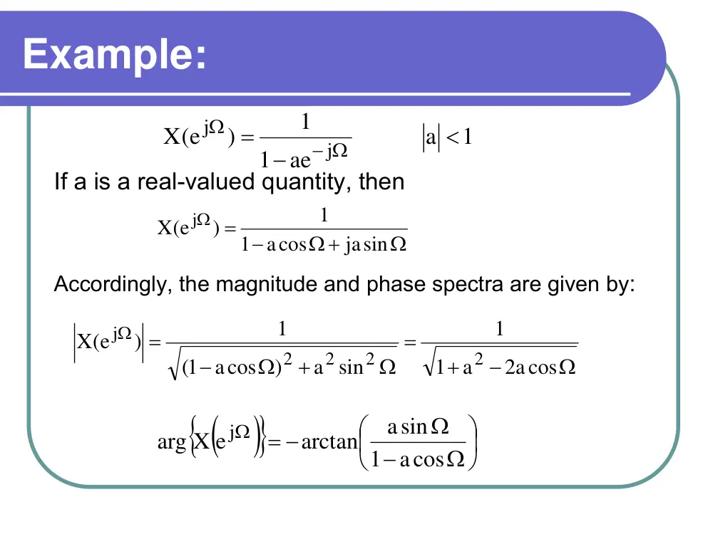Example: Find the DTFT of the exponential sequence Solution a u[n] x[n] n = ∑ ∑ ∞ = − Ω ∞ = −∞ = Ω Ω = = 0 n n j n n n j- j ) (ae x[n e ] ) e( X 1 a ae 1 1 ) X e( j j < − = − Ω Ω Example: If a is a real-valued quantity, then Accordingly, the magnitude and phase spectra are given by: 1 a ae 1 1 ) X e( j j < − = − Ω Ω jasin 1 acos 1 ) X e( j Ω Ω + − = Ω Ω − + = Ω + Ω − = Ω 2acos a 1 1 a sin ) acos 1( 1 ) X e( 2 2 2 2 j ( ) { } ⎟ ⎠ ⎞ ⎜ ⎝ ⎛ Ω − Ω Ω = − 1 acos asin arctan arg X e j 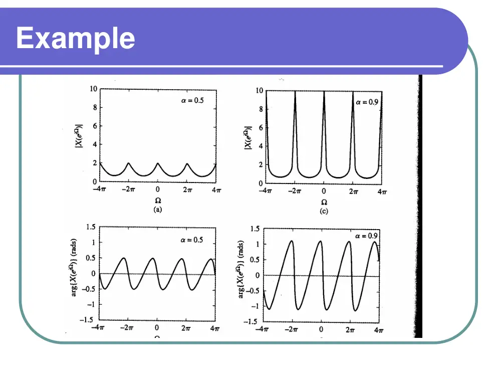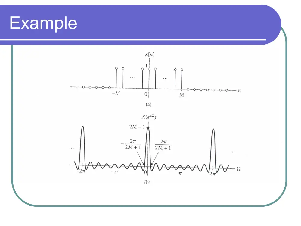Example Example 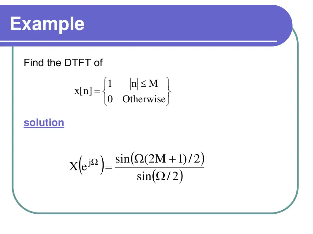Find the DTFT of solution ⎭ ⎬ ⎫ ⎩ ⎨ ⎧ ≤ = Otherwise 0 M n 1 [n] x ( ) ( ) ( /2) sin 2 /)1 (2M sin X e j Ω + Ω Ω = Example Example Find the DTFT of the following time-domain signal Answer ⎭ ⎬ ⎫ ⎩ ⎨ ⎧ ≤ ≤ = Otherwise 0 9 n 0 2 x[n] n ( ) Ω − Ω − Ω − − = j j10 10 j 2e 1 e 2 1 X e Properties of the DTFT 1. Linearity and Symmetry Properties The linearity property is used to find Fourier representations of signals that are constructed as sums of signals whose representations are already known ) bY e( ) aX e( ) Z e( by[n] ax[n] [z n] j j j DTFT Ω Ω Ω + = ⎯⎯ → ← + = Properties of the DTFT 2. Symmetry Properties: Real and Imaginary Signals a. For real-valued signals b. For Imaginary-valued signals ) X e( ) e( X j j − Ω Ω ∗ = ) X e( ) e( X j j − Ω Ω ∗ = − Properties of the DTFT 3. Convolution Property A similar property, to that of continuous non- periodic signals, holds for discrete-time non periodic signals The proof of this result closely parallels that of the continuous-time case. ) )Y e( X e( ) Z e( [y n] x[n] [z n] j j j DTFT Ω Ω Ω = ⎯ ⎯⎯ → ← ∗ = Properties of the DTFT 4. Shifting Property Where n0 is an integer value. For n0=1, then ) X e( e n ] x[n j j n DTFT 0 0 Ω − Ω ⎯ ⎯⎯ → ← − ) X e( e ]1 x[n j j DTFT Ω − Ω ⎯ ⎯⎯ → ← − Properties of the DTFT The shifting property can be used to determine the Frequency response of a discrete-time signal represented by a difference equation Taking the DTFT of both sides of this equation, we obtain ∑ ∑ = = − = − M k 0 k N k 0 k k] b x[n k] [y n a ∑ ∑ = Ω − = Ω − Ω Ω Ω = = N 0 k k j k M 0 k k j k i j j ) e( a ) e( b ) e( X ) Y e( ) H e( Example Find the difference corresponding to the system with frequency response Answer 3y[n]+2y[n-1]-3y[n-3]=x[n]+2x[n-2] Ω − Ω − Ω − Ω − + + = 3j j 2j j 3e 2e 3 2e 1 ) H e( Properties of the DTFT 5. Multiplication by n ) X e( x[n] jΩ ↔ [ ] Ω ↔ Ω d ) jd X e( nx[n] j Properties of the DTFT 6. Multiplication Property The multiplication property defines the Fourier representation of a product of discrete-time signals. If x[n] and z[n] are discrete-time nonperiodic signals, then the DTFT of the product y[n] = x[n ]z[n] is given by the convolution of the their DTFT's and multiplication by 1/2π. ) Z e( ) 2 X e( 1 [z n] x[n] [y n] j j DTFT Ω Ω ⊗ π ⎯ ⎯⎯ → ← ⋅ = Inverse of DTFT by Partial fraction expansion Example Find the Inverse DTFT of Ω − Ω − − Ω Ω − + − = 2j j j j 6 e 1 6 e 1 1 6 e 5 5 ) e( X ⎟ ⎠ ⎞ ⎜ ⎝ ⎟⎛ − ⎠ ⎞ ⎜ ⎝ ⎛ + − = − + − = − Ω Ω − Ω − Ω − Ω − − Ω Ω j j j 2j j j j 3 e 1 1 2 e 1 1 6 e 5 5 6 e 1 6 e 1 1 6 e 5 5 ) X e( Example Using Partial Fraction Expansion Then ⎟⎠ ⎞ ⎜⎝ + ⎛ − ⎟⎠ ⎞ ⎜⎝ ⎛ + = − Ω Ω − Ω j j j 3e 1 1 1 2 e 1 1 4 ) e( X 1( /3) u[n] 4( 1/ 2) u[n] x[n] n n + − = Example Find the frequency and impulse responses of the discrete-time system described by the following difference equations: y[n-2] + 5y[n-1] + 6y[n] = 8x[n - 1] + 18x[n] Answer 6 5e ) e( 18 8e ) H e( j 2 j j j + + + = − Ω Ω − − Ω Ω ( 1/ 2) u[n] 2 1( / 4) u[n] h[n] n n + − = Parseval’s Theorem for Energy Signals ∫ ∑ π π − Ω ∞ = =−∞ Ω π = ) d X e( 2 1 x[n] 2 j n n 2 Example Let Use Parseval's theorem to evaluate the energy of x[n] Solution Using the DTFT, we have It follows that the energy of x[n]=W/π n sin(Wn) x[n] π = ⎭ ⎬ ⎫ ⎩ ⎨ ⎧ < Ω ≤ π Ω ≤ = ⎯ ⎯⎯ → ← Ω W 0 W 1 ) X e( x[n] j DTFT