EECE 340 Chapter 3, Fall 2011

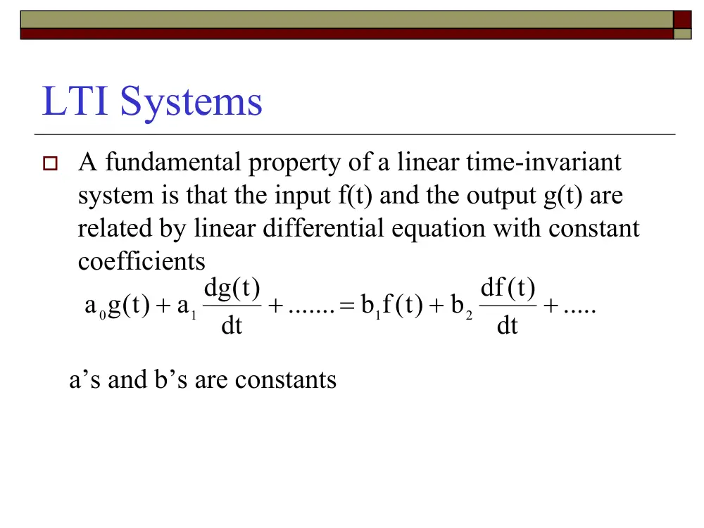
Chapter 3 Linear Time-Invariant Systems Chapter Outlines � In this chapter, we will discuss linear time-invariant (LTI) systems. These are systems that are both linear and time-invariant. We will see that an LTI system has an input-output relationship described by a convolution. LTI Systems � A fundamental property of a linear time-invariant system is that the input f(t) and the output g(t) are related by linear differential equation with constant coefficients a’s and b’s are constants ..... dt )t( b df )t( b f ....... dt a dg )t( g )t( a 2 1 1 0 + + = + + Input-Output System Relationship � we examine several methods for describing the relationship between the input and output signals of linear time-invariant (LTI) systems. � In characterizing the behavior of systems, we follow two main plans of analysis: 1. 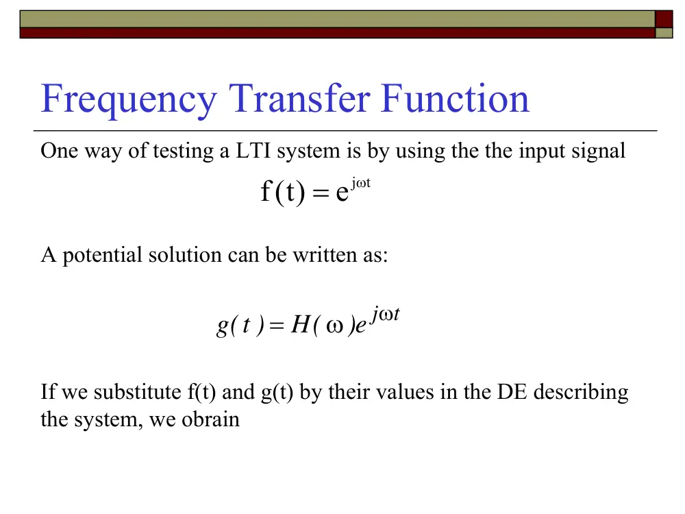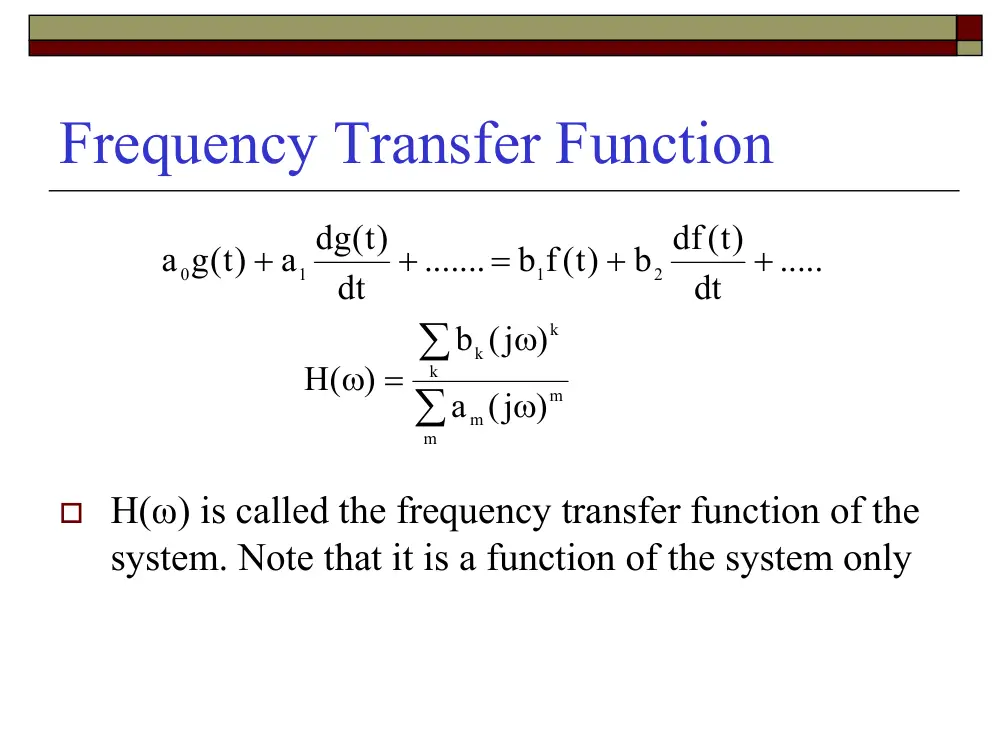Frequency domain (discussed in short now and detailed later) 2.Time domain (objective of this chapter) Frequency Transfer Function One way of testing a LTI system is by using the the input signal A potential solution can be written as: If we substitute f(t) and g(t) by their values in the DE describing the system, we obrain je t )t( f ω = e) j t H( g t( ) ω ω = Frequency Transfer Function ..... dt )t( b df )t( b f ....... dt a dg )t( g )t( a 2 1 1 0 + + = + + ∑ ∑ ω ω = ω m m m k k k ) j( a ) j( b ( ) H � H(ω) is called the frequency transfer function of the system. 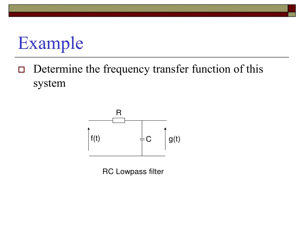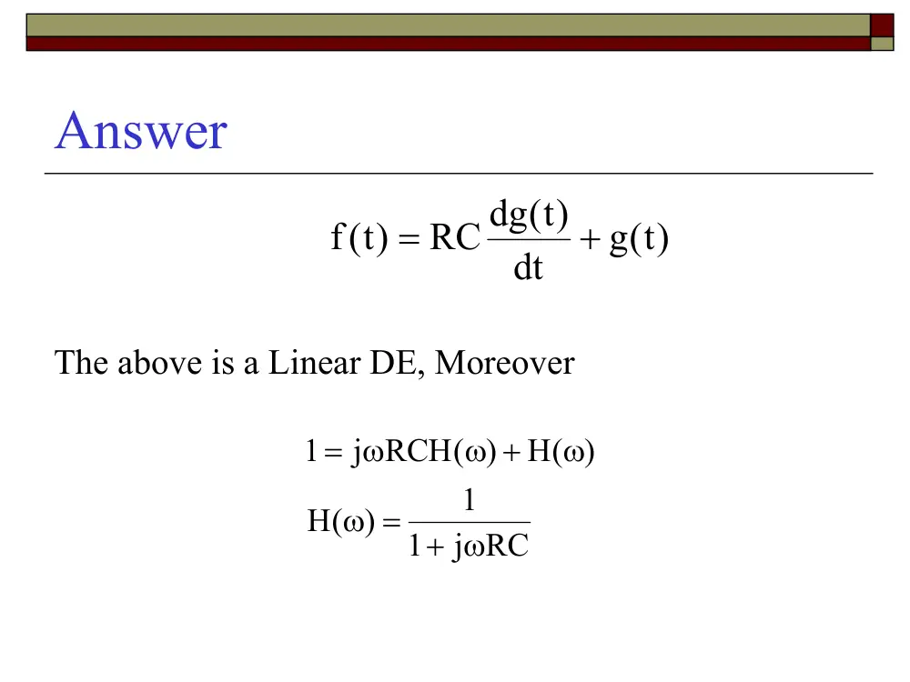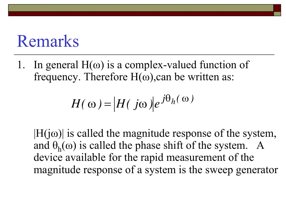Note that it is a function of the system only Example � Determine the frequency transfer function of this system R C f(t) g(t) RC Lowpass filter Answer g )t( dt RC dg )t( )t( f + = The above is a Linear DE, Moreover j RC 1 1 ( ) H H( ) j RCH( ) 1 = + ω ω ω ω + = ω Remarks 1. In general H(ω) is a complex-valued function of frequency. Therefore H(ω),can be written as: |H(jω)| is called the magnitude response of the system, and θh(ω) is called the phase shift of the system. A device available for the rapid measurement of the magnitude response of a system is the sweep generator ) )e j h( H( j ) H( ω θ ω ω = Impulse Response � As it was said earlier, that the system can be represented either in time or frequency domains by impulse response (The response of the system when the input is an impulse function � Mathematically speaking, if the system input is δ(t) and the corresponding output is g(t), then g(t)=F{δ(t)}. Example � Determine the impulse response of the system shown below ∑ Integrator Delay: + + f t( ) g t( ) y t( ) t 0 Example � Answer: h(t)=u(t)-u(t-t0) t0 t h t( ) 1 The Convolution Integral � The output of a continuous-time LTI system may also be determined solely from knowledge of the input and the system's impulse response LTI System h t( ) x t( ) y t( ) The Convolution Integral � The input-output relationship is given by the integral equation known as the convolution integral h(t) is the impulse response of the system, x(t) is the input signal, and y(t) is the output signal. The above integral is the convolution integral and it is denoted by: ∫ +∞ −∞ τ − τ τ = )d x( )h t( )t( y y t x t h t ( ) ( ) ( ) = ∗ The Convolution Integral � The convolution integral can also be written as: τ − τ ∫ τ = τ − τ ∫ τ = ∞ + ∞ − +∞ ∞ − )d t( h( x) )t( y )d t( x( h) y )t( The Convolution Integral If h(t) is causal then and x(t)=0 for t<0, then ⇒ ⎪⎩ ⎪⎨ ⎧ < τ − τ = < = t for 0 ) h t( 0 t for 0 )t( h τ − τ ∫ τ = −∞ )d t( x( h) )t( y t τ − τ ∫ τ = )d t( x( h) )t( y t 0 Properties of the Convolution Integral 1. Commutative The Convolution integral is symmetric with respect to x(t) and h(t) x )t( y )t( y )t( x )t( ∗ = ∗ τ − τ τ τ = − τ τ ∫ ∫ +∞ ∞ − +∞ −∞ )d t(x) (y )d t(y) (x Properties of the Convolution Integral 2. Distributive The Convolution integral satisfies the following property )t( f )t( f )t( f )t( f t( )] f )t( f[ )t( f 3 1 2 1 3 2 1 ∗ + ∗ = + ∗ Properties of the Convolution Integral 3. Associative The Convolution integral satisfies the following property t( ) f t( )] f t( ) [ f t( )] f t( ) t( ) [ f f 3 2 1 3 2 1 ∗ ∗ = ∗ ∗ Example If h(t)=Asin(πt)u(t) and x(t)=δ(t)-δ(t-2), detrmine y(t)=x(t)*h(t). Example 1: Solution h(t) t (1) 2 x(t) t (2) y(t) t (2) (1) Example 2 If x(t) = u(t-1) – u(t-3) and h(t) = u(t) – u(t-2), determine y(t)=x(t)*h(t) Example 2: Solution ⎪ ⎪ ⎭ ⎪⎪ ⎬ ⎫ ⎪ ⎪ ⎩ ⎪⎪ ⎨ ⎧ > ≤ ≤ − ≤ ≤ − < = 5 t 0 5 t 3 t 5 3 t 1 1 t 1 t 0 y )t( Example 3 Let the impulse response of an LTI system be given by: h(t) = u(t - 1) - u(t - 4). Find the output of this system in response to the input x(t) = u(t) + u(t - 1) - 2u(t - 2). Example 3: Solution ⎪ ⎪ ⎪ ⎪ ⎭ ⎪ ⎪ ⎪ ⎪ ⎬ ⎫ ⎪ ⎪ ⎪ ⎪ ⎩ ⎪ ⎪ ⎪ ⎪ ⎨ ⎧ ≥ ≤ < − ≤ < − > ≤ ≤ < − ≤ < − < = 6 t 0 6 t 5 2t 12 5 t 4 t 7 4 t 3 3 3 t 2 3 t 2 2 t 1 1 t 1 t 0 y )t( Interconnections of LTI Systems � In this section, we develop the relationships between the impulse response of an interconnection of LTI systems and the impulse responses of the constituent systems. Parallel Connection of LTI Systems Consider two LTI systems with impulse responses h1(t) and h2(t) connected in parallel, as shown below � h1(t) � h2(t) Parallel Connection of LTI Systems � The output of this connection of systems, y(t), is the sum of the outputs of the two systems: x(t) y(t) � Mathematically, the preceding result implies that convolution possesses the distributive property )t( h )t( h 2 1 + Cascade Connection of Systems � Consider next the cascade connection of two LTI systems, as illustrated below h1(t) h2(t) � Let y(t) be the output of the first system and therefore the input to the second system in the cascade, and let z(t) be the output of the second system x(t) z(t) y(t) Cascade Connection of Systems )t( h y )t( )t( z )t( h x )t( )t( y 2 1 ∗ = ∗ = The above implies t( )} h )t( {h x )t( )t( z 2 1 ∗ ∗ = )t( h )t( h 2 1 ∗