EECE 340 Chapter 14, Fall 2011

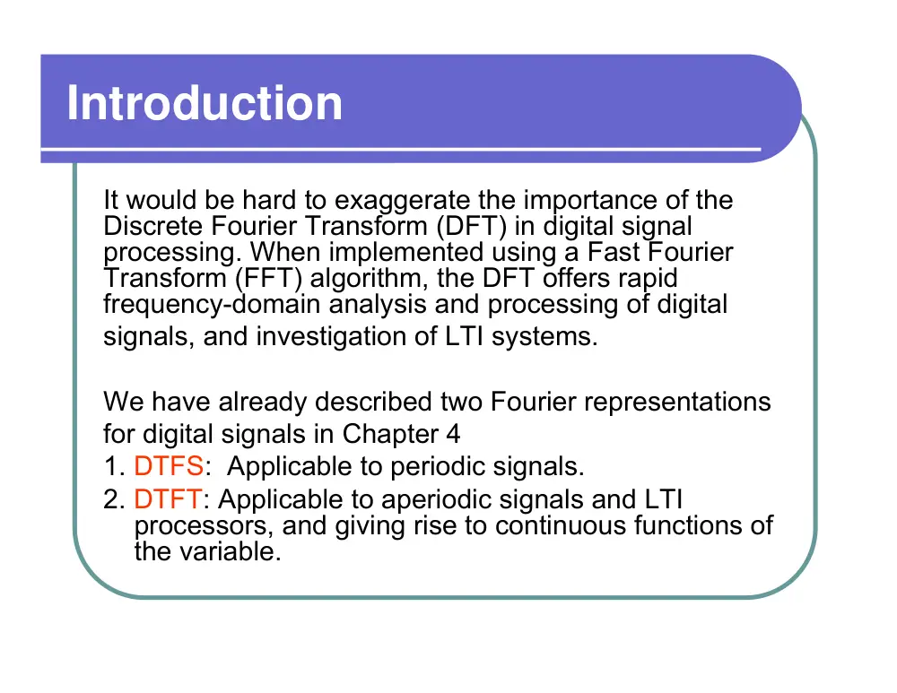
CHAPTER 14 The Discrete and Fast Fourier Transforms Introduction It would be hard to exaggerate the importance of the Discrete Fourier Transform (DFT) in digital signal processing. When implemented using a Fast Fourier Transform (FFT) algorithm, the DFT offers rapid frequency-domain analysis and processing of digital signals, and investigation of LTI systems. We have already described two Fourier representations for digital signals in Chapter 4 1. DTFS: Applicable to periodic signals. 2. DTFT: Applicable to aperiodic signals and LTI processors, and giving rise to continuous functions of the variable. 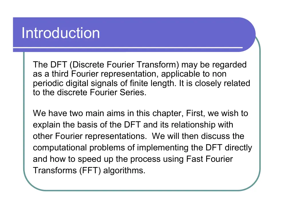Introduction The DFT (Discrete Fourier Transform) may be regarded as a third Fourier representation, applicable to non periodic digital signals of finite length. It is closely related to the discrete Fourier Series. We have two main aims in this chapter, First, we wish to explain the basis of the DFT and its relationship with other Fourier representations. We will then discuss the computational problems of implementing the DFT directly and how to speed up the process using Fast Fourier Transforms (FFT) algorithms. 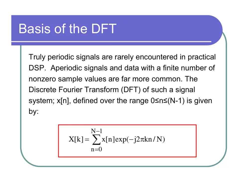Basis of the DFT Truly periodic signals are rarely encountered in practical DSP. Aperiodic signals and data with a finite number of nonzero sample values are far more common. 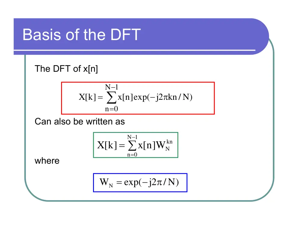The Discrete Fourier Transform (DFT) of such a signal system; x[n], defined over the range 0≤n≤(N-1) is given by: ∑ − = π − = 1 N n 0 kn / N) 2j x[n]exp( X[k] Basis of the DFT The DFT of x[n] Can also be written as where ∑ − = π − = 1 N n 0 kn / N) 2j x[n]exp( [k] X ∑ − = = 1 N 0 n kn x[n]WN [k] X / N) 2j exp( WN π − = Basis of the DFT Note that the spectral coefficients X[k] are evaluated for 0≤k≤(N-1). . 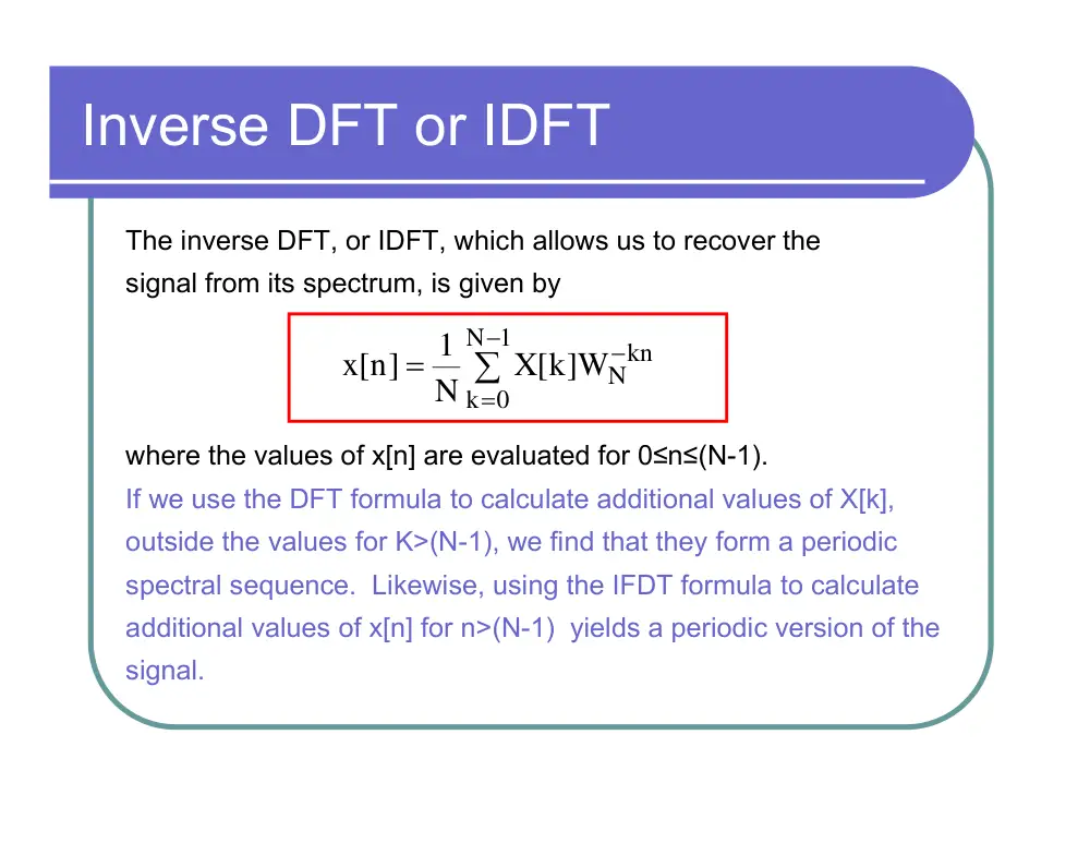Inverse DFT or IDFT The inverse DFT, or IDFT, which allows us to recover the signal from its spectrum, is given by where the values of x[n] are evaluated for 0≤n≤(N-1). If we use the DFT formula to calculate additional values of X[k], outside the values for K>(N-1), we find that they form a periodic spectral sequence. Likewise, using the IFDT formula to calculate additional values of x[n] for n>(N-1) yields a periodic version of the signal. ∑ − = − = 1 N 0 k X[k]WNkn N 1 x[n] Basis of the DFT � We therefore see that the DFT and IDFT both represent a finite-length sequence as one period of a periodic sequence. In effect the DFT considers an aperiodic signal x[n] to be periodic for the purposes of computation. � Note that the only difference between the DFT and the IDFT is the scaling factor of (1/N), and a sign change in the exponent. Therefore, if we have an algorithm for computing the DFT, it is a simple matter to modify it to compute the IDFT. This is a direct consequence of the symmetry between time and frequency domains Properties of the DFT 1. Periodicity x[n] = x[n+N] for all n and X[k] = X[k+N] for all k The property can also be interpreted by evaluating the indices modulo-N. 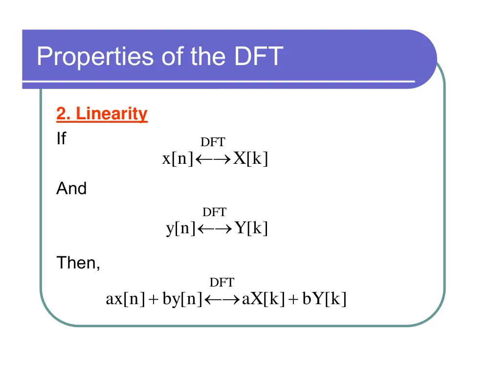Properties of the DFT 2. Linearity If And Then, X[k] x[n] DFT ←→ Y[k] [y n] DFT ←→ bY[k] aX[k] by[n] ax[n] DFT + ←→ + Properties of the DFT 3. Time Shifting If Then X[k] x[n] DFT ←→ 0 kn N ( j2kn0 / N) DFT 0 X[k]W X[k e] n ] x[n = ←→ − − Properties of the DFT 4. Circular Convolution What happens when we multiply two DFT's together Y[k]=X[k]H[k], where X[k] is the DFT of x[n] and H[k] is the DFT of h[n] when 0≤k≤(N-1) ? Answer Using the IDFT synthesis formula for y[n], we obtain ∑ − = π = 1 N 0 k N kn j2 X[k]H[k e] N 1 [y n] Circular convolution Using the fact We obtain ∑ − = π = 1 N 0 k N kn j2 X[k]H[k e] N 1 n] [y ∑ − = π − = 1 N 0 m N km j2 h[m e] [k] H ∑ ∑ − = π − = π − ⎟ ⎟ ⎠ ⎞ ⎜ ⎜ ⎝ ⎛ = 1 N 0 k N kn j2 1 N 0 m N km j2 e h[m e] X[k] N 1 n] [y ∑ ∑ − = − π − = = 1 N 0 k N k(n m) j2 1 N m 0 X[k e] N h[m] 1 [y n] Circular convolution where we can reduce the second summation into Then The above is called circular convolution, and it is denoted by: ∑ ∑ − = − π − = = 1 N 0 k N k(n m) j2 1 N m 0 X[k e] N h[m] 1 n] [y [ ] ∑ − = − π = − 1 N 0 k N k(n m) 2 j mod N X[k e] N 1 m) (n x [ ] N N m m h m x n y n mod 1 0 ) [ ] ( [ ] − = ∑ − = h[n] x[n] [y n] ⊕ = Steps for Circular convolution computation Steps for cyclic convolution are the same as the usual convolution, except all index calculations are done "mod N" = "on the wheel" . Step 1: construct two circles as shown below Steps for Circular convolution computation Step 2: Divide each circle into N equally spaced arcs Steps for Circular convolution computation Step 3: Place the first sequence on the outer circle in the contour-clockwise direction and the other sequence on the inner circle in the clockwise direction (inverted). for k=0; multiply the overlapping numbers and add. X[0] X[1] X[2] X[3] h[0] h[3] h[2] h[1] Steps for Circular convolution computation Step 4: for k=1, rotate the outer circle clockwise one unit. Again, multiply the overlapping numbers and add. Step5: Repeat the same steps until k=N-1 Properties of the DFT 5. Modulation If Then X[k] x[n] DFT ←→ Y[k] n] [y DFT ←→ ∑ − = − ⎯→ ← 1 N m 0 m] X[m]Y[k N 1 x[n] [y n] THE FAST FOURIER TRANSFORM (FFT) BASIS OF THE FFT Highly efficient algorithms for computing the DFT were first developed in the 1960s. Collectively, known as Fast Fourier Transforms (FFTs), they all rely upon the fact that the standard DFT involves redundant calculation. The DFT of an N-length signal is given by: where Wn=exp(-j2π/N) and X[k] are evaluated for 0≤k≤(N-1). It turns out that the same values in the sum are calculated many times as the computation proceeds - particularly if the transform is lengthy. This is because Wn is a periodic function with a limited number of distinct values. The same is true of the IDFT. It is the aim of FFT algorithms to eliminate the redundancy ∑ − = π − = 1 N n 0 kn / N) 2j x[n]exp( [k] X ∑ − = = 1 N 0 n kn x[n]WN X[k]