EECE 340 Chapter 4, Fall 2011

Chapter 4 The Laplace Transform The Laplace Transform 1. In this lesson, we'll introduce the Laplace Transform. The Laplace Transform is useful in a number of different applications. Using the Laplace Transform, differential equations can be solved algebraically. 2. We can use pole/zero diagrams from the Laplace Transform to determine the frequency response of a system and whether or not the system is stable. 3. We can transform more signals than we can with the Fourier Transform, because the Fourier Transform is a special case of the Laplace Transform. 4. The Laplace Transform is used for analog circuit design. 5. 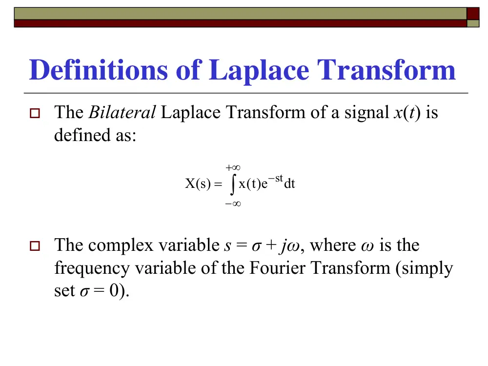The Laplace Transform is used in Control Theory and Robotics Definitions of Laplace Transform � The Bilateral Laplace Transform of a signal x(t) is defined as: � The complex variable s = σ + jω, where ω is the frequency variable of the Fourier Transform (simply set σ = 0). 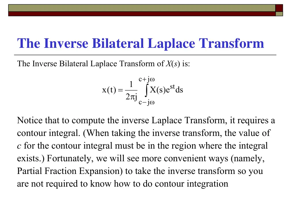∫ +∞ ∞ − − = dt e)t( x )s( X st The Inverse Bilateral Laplace Transform The Inverse Bilateral Laplace Transform of X(s) is: Notice that to compute the inverse Laplace Transform, it requires a contour integral. 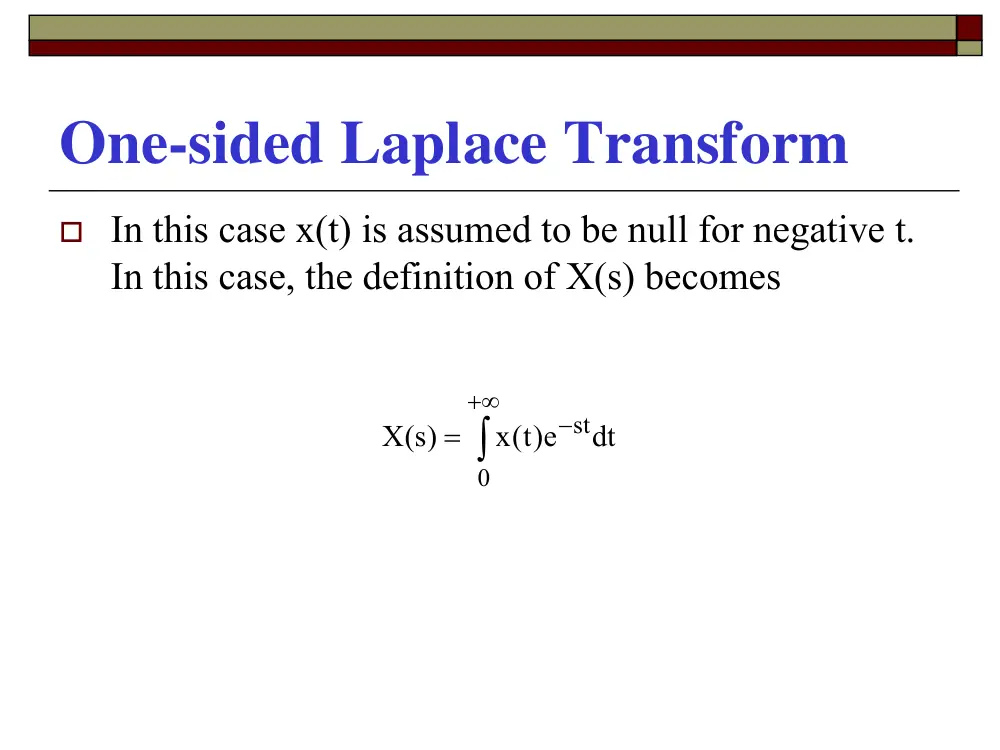(When taking the inverse transform, the value of c for the contour integral must be in the region where the integral exists.) Fortunately, we will see more convenient ways (namely, Partial Fraction Expansion) to take the inverse transform so you are not required to know how to do contour integration ∫ ω + − ω π = j c j c stds e)s( X 2 j 1 x )t( One-sided Laplace Transform � In this case x(t) is assumed to be null for negative t. 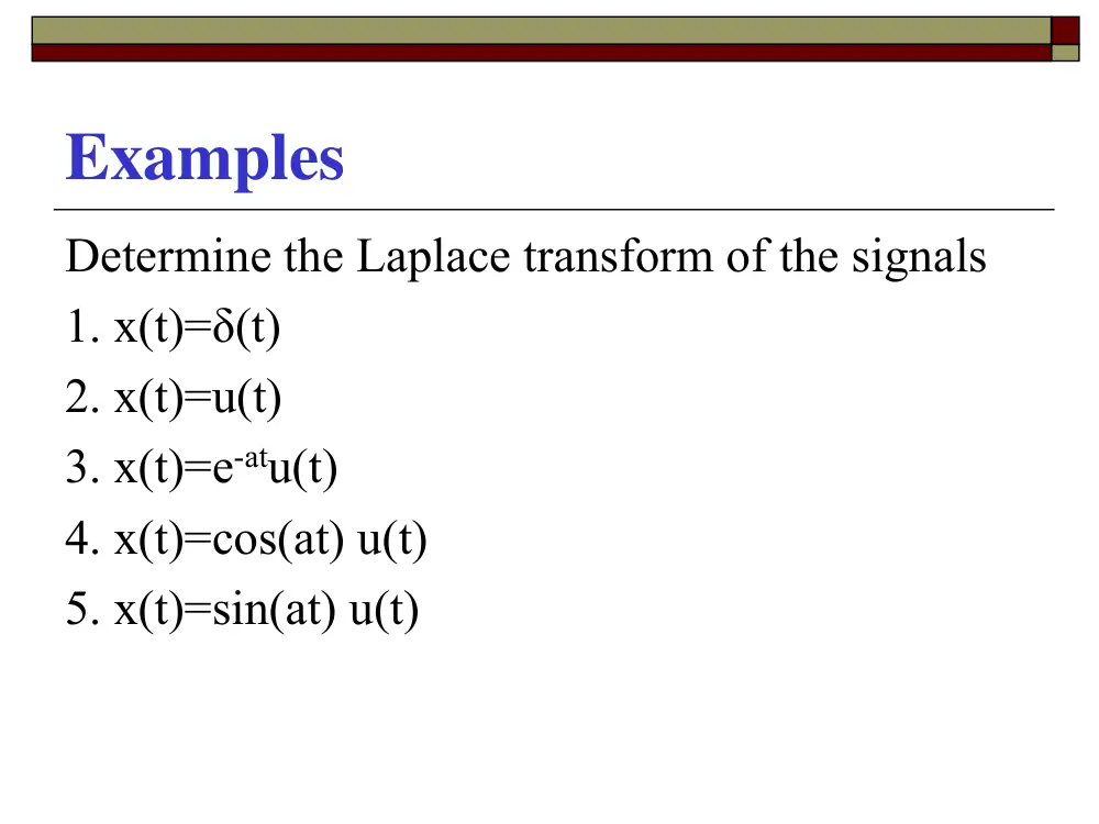In this case, the definition of X(s) becomes ∫ +∞ − = 0 stdt e)t( x X )s( Examples Determine the Laplace transform of the signals 1. x(t)=δ(t) 2. x(t)=u(t) 3. x(t)=e-atu(t) 4. x(t)=cos(at) u(t) 5. 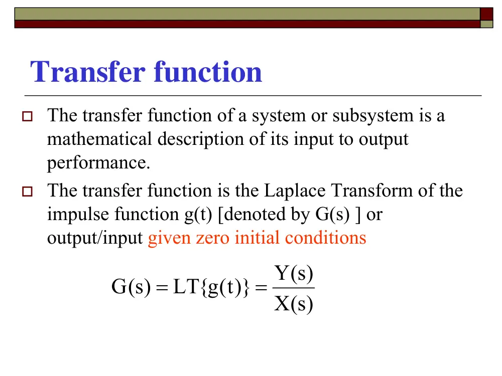x(t)=sin(at) u(t) Properties of the LT � Linearity � Time shifting � Differentiation � Integral � Multiplication by t � Convolution � Initial Value Theorem � Final Value Theorem Transfer function � The transfer function of a system or subsystem is a mathematical description of its input to output performance. 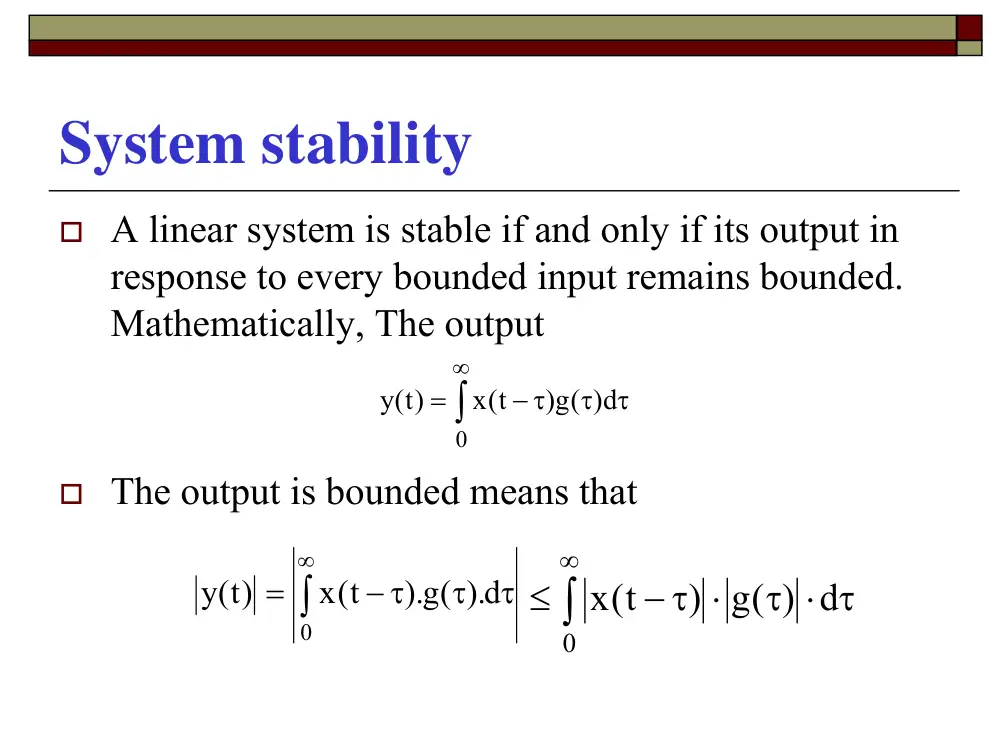� The transfer function is the Laplace Transform of the impulse function g(t) [denoted by G(s) ] or output/input given zero initial conditions X )s( Y )s( LT{g t( )} G )s( = = System stability � A linear system is stable if and only if its output in response to every bounded input remains bounded. 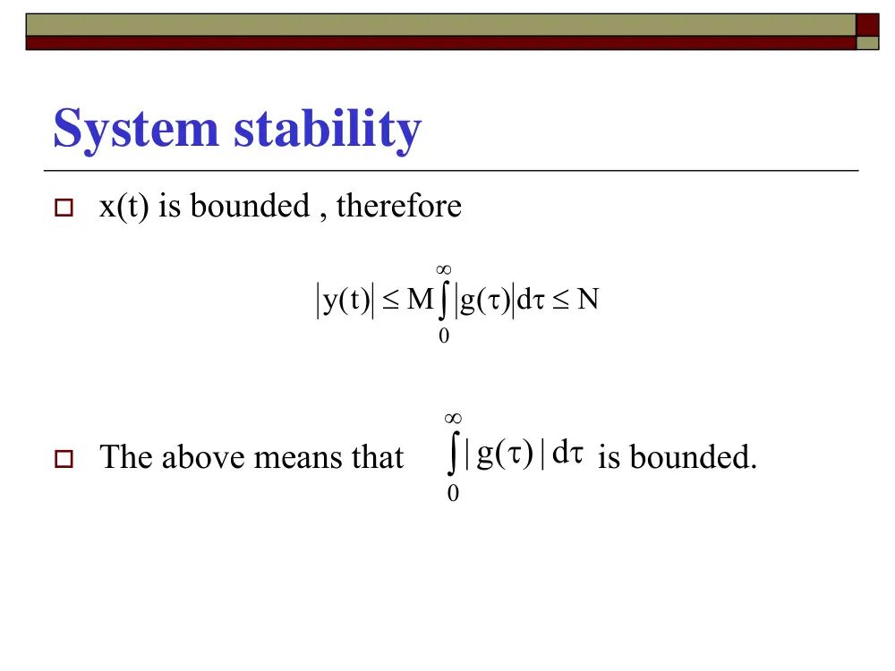Mathematically, The output � The output is bounded means that ∫ ∞ τ τ − τ = 0 )g( )d x t( )t( y ∫ ∞ τ τ − τ = 0 ).g( ).d x t( y )t( ∫ ∞ τ ⋅ τ − τ ⋅ ≤ 0 ) g( ) d x t( System stability � x(t) is bounded , therefore � The above means that is bounded. ∫ ∞ τ ≤ τ ≤ 0 N g( ) d M )t( y ∫ ∞ τ τ 0 |) d | g( System stability in the s-domain � A linear system is stable if and only if all poles of the transfer function lie in the left-half of the complex-plane. � The above means that Q(s) has no roots in the RHP and on the jω axis Q )s( P )s( X )s( Y )s( = System stability in the s-domain In order to determine the system stability in the s-domain, 2 steps are needed � Determine the closed loop transfer function � Check for the location of the poles of Y(s)/X(s) or Zeros of Q(s) Transfer Function computation � In this section, we will try to determine the transfer function of a LTI system represented by either a DE or by block diagram. Example 1 � An LTI system, whose output is c(t) and input r(t), is represented by the following DE. Determine the Transfer function of this system )t(r 2 2c )t( )t(c 3 c )t( = + + � �� Example 2 Determine the transfer function of the following system Example 3 Determine the transfer function of the following system C(s) The transfer function of the above system is: G )s( H )s( 1 G )s( )s( R C )s( = + Example 3. Important Notation � G(s) the forward transfer function. � H(s) the feedback transfer function. � In many cases, H(s) = 1, and the system is called a unity feedback system. � In this case, E(s) is called the error signal. � G(s)/[1+G(s)H(s)] is called the closed-loop transfer function. � {G(s)H(s)} is the open-loop transfer function. Example 4 Determine the transfer function of the following system Example 5 General Gain Formula for Signal Flow Graphs (Mason’s rule) For an LTI system, the TF is computed as follows Where M is the gain between yin and yout , yout is the output node variable, yin is the input node Variable, N is the total number of forward paths, and Mk is the gain of the Kth forward path. ∑ = ∆ ∆ = = N 1 k k k in out M y y M General Gain Formula for Signal Flow Graphs (Mason’s rule) ∆ =1 – (sum of all individual loop gains) + (sum of gain products of all possible combinations of 2 non-touching loops) - (sum of gain products of all possible combinations of 3 non-touching loops) + ….. ∆k = the ∆ for that part of the signal flow graph which is non-touching with the Kth forward path. Example 5 2 4 4 1 2 3 2 3 2 1 1 2 1 4 1 3 1 2 G H G G G G H G G G 1 G G H G G G G G R C + + + + + + = Check for the location of the poles of Y(s)/X(s) A transfer function of the form An analytical procedure for determining the exact location of the poles of the TF (n>3) function is impossible. As we need to know the stability of the system, determining the number of roots in each half of the complex plane is sufficient. 0 1 n 1 n 1 n n 0 1 m 1 m 1 m m b b s .... s b b s a a s .... s a a s X )s( Y )s( + + + + + + + + = − − − − Routh and Hurwitz criteria (RH) � This theory gives an affirmative answer for the absolute stability, but it does not give any information about the relative stability of the system. � It is based on the coefficients of the polynomial Q(s). � Necessary conditions but not sufficient 1. all b’s have the same sign. 2. None is zero. 0 .............. 0 1 1 1 = + + + + − − b b s s b b s n n n n The RH Table n s nb nb −2 −4 nb nb −1 nb −3 nb −5 −1 ns −2 ns −3 ns 1c 2c 3c d3 d1 2 d 1 g 1h 1s 0s RH Table Coefficients The R-H criterion states that the number of polynomial roots with positive real part equals the number of coefficient sign changes in the first column of the coefficient array we have developed 1 3 2 1 1 − − − − − = n n n n n b b b b b c 1 5 4 1 2 − − − − − = n n n n n b b b b b c 1 1 2 3 1 1 c c b c b d n n − − − = Where The R-H criterion states that the number of polynomial roots with positive real part equals the number of coefficient sign changes in the first column of the coefficient array we have developed. 1 3 2 1 1 − − − − − = n n n n n b b b b b c 1 5 4 1 2 − − − − − = n n n n n b b b b b c 1 1 2 3 1 1 c c b c b d n n − − − = Example: 1 pole in RHP, system is unstable . 2 1 2) 1)( ( 1 ( ) 2 − + = + − = s s s s s Q 2 0 1 2 1 0 1 2 − − s s s Example: (Two sign changes ; 2 poles in RHP), System is unstable. 800 200s 88s 14s 2s s 20 17s 12s 3s )s( Q 2 3 4 5 2 3 + + + + + − + − = 1 14 200 2 88 800 -30 -200 0 74.7 800 121 0 800 5s 4 s 3s s2 1s 0s Example: Two RHP roots. 1 0 3 6 2 3 1 3 6 0 3 2 ( ) 0 1 6 2 2 3 1 0 2 1 2 3 4 5 s s s nb s s s − − − δ δ δ δ δ is very small number δ 1 2s 6s 3s 2s s )s( Q 2 3 4 5 + + + + + = Example : Auxiliary Polynomial A(s)= 8 12s 6s 3s s )s( Q 2 3 4 + + + + = 8 0 4 0 0 0 8 2 0 12 3 8 6 1 0 1 1 2 3 4 s s s s s s 8 2 2 + s s ds dA s 4 ( ) = roots of A(s) are roots of Q(s).S ystem is unstable 2j s;4 ,8 then s 2s )s( A 2 2 = ± = − ⋅ + = Example 8 20s 16s 4s 2s 5s 4s s )s( Q 2 3 4 5 6 7 + + + + + + + = State-Variable Representation of LTI Systems � The state variable and the state equation of a dynamic system are defined simply as a set of first-order differential equations relating the state variables among themselves and to the inputs � This representation is best done with the use of an example BU )t( AX )t( dt dX )t( + = Example A linear system has one input and one output. The input-output relation is defined by: where y(t) is the output signal and r(t) is the input signal. Write the state equations of this system )t(r 3 dt 2 dr )t( 6y )t( dt 5dy )t( dt 3d y )t( dt d y )t( 2 2 3 3 + = + + + Steps 1. Put the highest derivative on one side and the rest on the other sides. Remember that for stability the derivative order of the output is greater than or equal to that of the input. 2. Apply number of integrators equal to that of the order of the derivative of y(t). 3. Construct the block diagram 4. Deduce the state equations. Solution Step 1 )t(r 3 dt 2 dr )t( 6y )t( dt 5dy )t( dt 3d y )t( dt d y )t( 2 2 3 3 + + − − = − step 2 step 3 ∫∫∫ ∫∫ ∫∫∫ ∫ ∫∫ + + − − = − dt )t(r 3 dt )t(r 2 y )t( dt 6 y )t( dt 5 3 y )t( dt )t( y -3 -5 -6 3 2 y(t) ∫ ∫ ∫ Step 4 Let be the outputs of the integrators. From the figure, we obtain Moreover, the output y(t) is given by: )t( t( ),X t( ),X X 3 2 1 )t( X )t( 3X )t( X dt )t( dX 2 1 / 1 1 + = − = )t(r 2 )t( X )t( 5X )t( X dt )t( dX 3 1 / 2 2 + + = − = )t(r 3 6X t( )t( X dt )t( dX 1 / 3 3 + = − = )t( X )t( y 1 = The above equations can be written in a matrix form )t(r 3 2 0 )t( X )t( X )t( X 0 0 6 1 0 5 0 1 3 X )t( )t( X )t( X )t( X 3 2 1 / 3 / 2 / 1 ⎥ ⎥ ⎥ ⎦ ⎤ ⎢ ⎢ ⎢ ⎣ ⎡ + ⎥ ⎥ ⎥ ⎦ ⎤ ⎢ ⎢ ⎢ ⎣ ⎡ ⎥ ⎥ ⎥ ⎦ ⎤ ⎢ ⎢ ⎢ ⎣ ⎡ − − − = = ⎥ ⎥ ⎥ ⎦ ⎤ ⎢ ⎢ ⎢ ⎣ ⎡ [ ] [ ] )t(r 0 )t( X )t( X )t( X 0 0 1 )t( y 3 2 1 + ⎥ ⎥ ⎥ ⎦ ⎤ ⎢ ⎢ ⎢ ⎣ ⎡ =