EECE 340 Chapter 5, Fall 2011

Chapter 5 Fourier Representation of Signals Introduction The study of signals and systems using sinusoidal representations is termed Fourier analysis, after Joseph Fourier (1768-1830) for his development of the theory. Fourier methods have widespread application beyond signals and systems, being used in every branch of engineering and science. 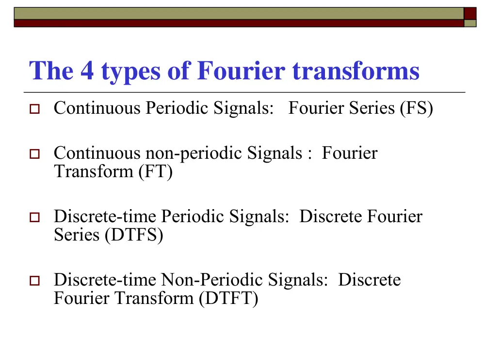There are four distinct Fourier representations, each applicable to a different class of signals, determined by the periodicity properties of the signal and whether the signal is discrete and or continuous in time The 4 types of Fourier transforms � Continuous Periodic Signals: Fourier Series (FS) � Continuous non-periodic Signals : Fourier Transform (FT) � Discrete-time Periodic Signals: Discrete Fourier Series (DTFS) � Discrete-time Non-Periodic Signals: Discrete Fourier Transform (DTFT) Fourier series � Let f(t) be a periodic signal with period T0 and frequency ω0. By using a Fourier series expansion, f(t) can be written as follows: � Where )t b sin(n )t a cos(n a )t( f 0 n n 1 n 1 0 n 0 ω + ω + = ∑ ∑ ∞ = ∞ = − ∫ = / 2 T T / 2 0 0 0 0 f t( ).dt T 1 a ,... 3,2,1 n .t dt f t( ).cosn T 2 a / 2 T T / 2 0 0 n 0 0 = ω = ∫ − ,... 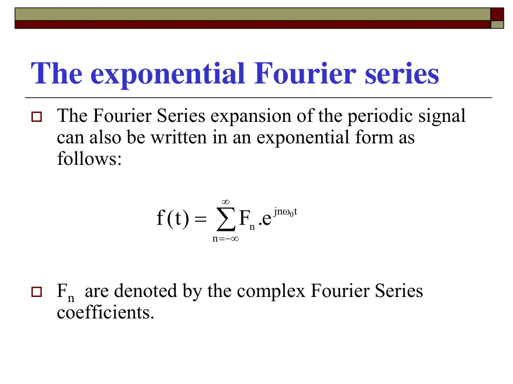3,2,1 n .t dt f t( ).sin n T 2 b / 2 T T / 2 0 0 n 0 0 = ω = ∫ − The exponential Fourier series � The Fourier Series expansion of the periodic signal can also be written in an exponential form as follows: � Fn are denoted by the complex Fourier Series coefficients. ∑ ∞ −∞ = ω = n t jn n 0 F e. 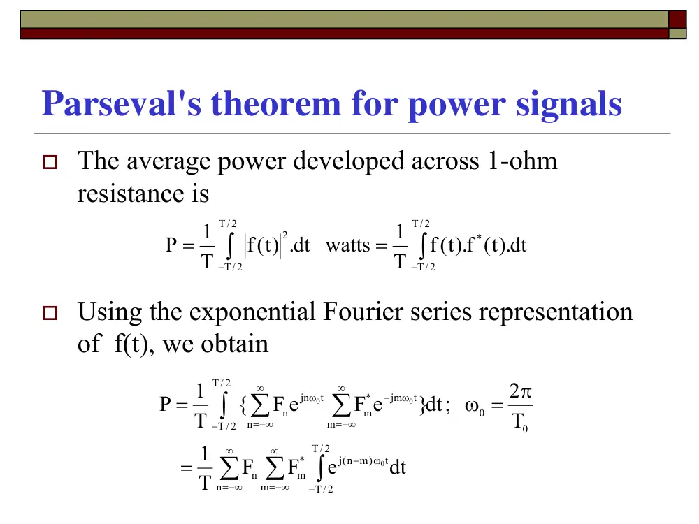)t( f Determination of Fn � Prove that ∫ − − ω = / 2 T / 2 T t jn 0 n 0 0 0 dt e)t( f T 1 F Example Derive the exponential Fourier Series of the following function: Answer: T / 2 f t( ) t − T / 2 T0 ⎟⎟ ⎠ ⎞ ⎜⎜ ⎝ ⎛ π ⎟⎟ ⎠ ⎞ ⎜⎜ ⎝ ⎛ π ⎟⎟ = ⎠ ⎞ ⎜⎜ ⎝ ⎛ π π = 0 0 0 0 n T T n T T n sin T AT T T sin n .n A F Parseval's theorem for power signals � The average power developed across 1-ohm resistance is � Using the exponential Fourier series representation of f(t), we obtain ∫ ∫ − − = = / 2 T / 2 T * / 2 T / 2 T 2 t( ).dt f t( ).f T 1 .dt watts )t( f T 1 P dt e F F T 1 T 2 }dt; F e F e { T 1 P / 2 T / 2 T t n m) (j m * m n n 0 0 m t jm * m / 2 T T / 2 n t jn n 0 0 0 ∫ ∑ ∑ ∑ ∫ ∑ − ω − ∞ −∞ = ∞ −∞ = ∞ −∞ = ω − − ∞ −∞ = ω = π ω = = 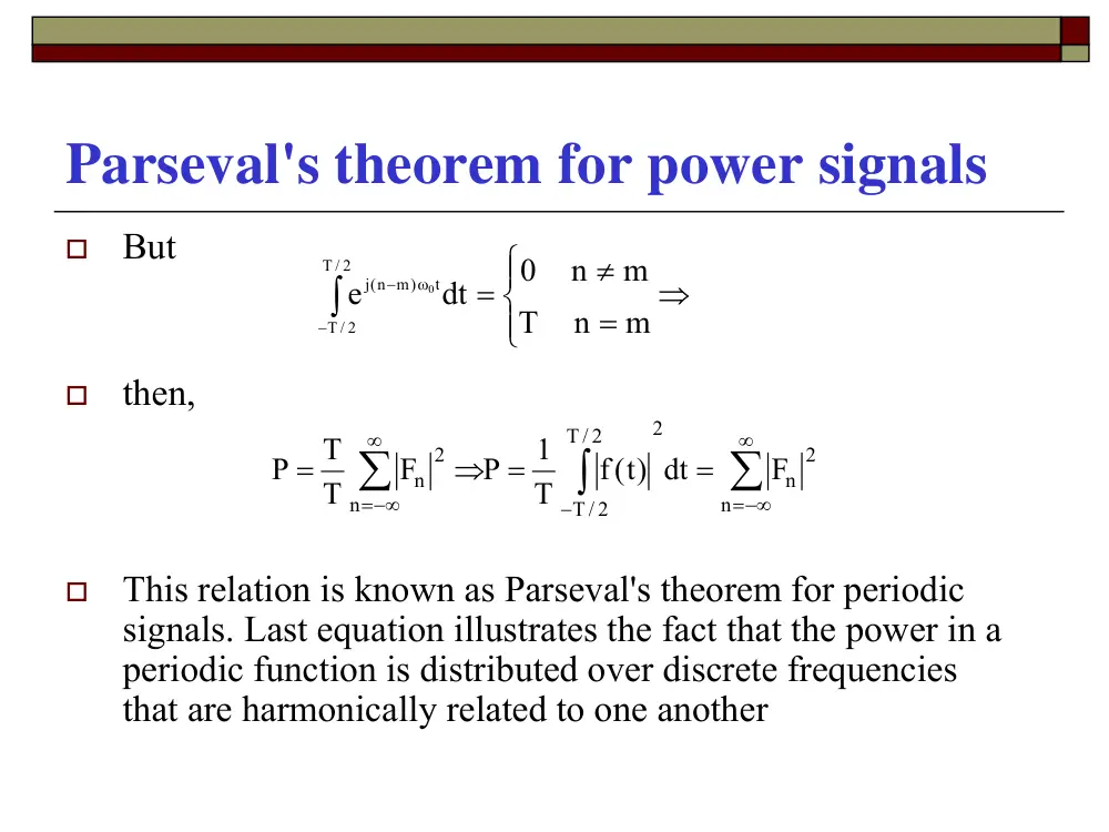Parseval's theorem for power signals � But � then, � This relation is known as Parseval's theorem for periodic signals. 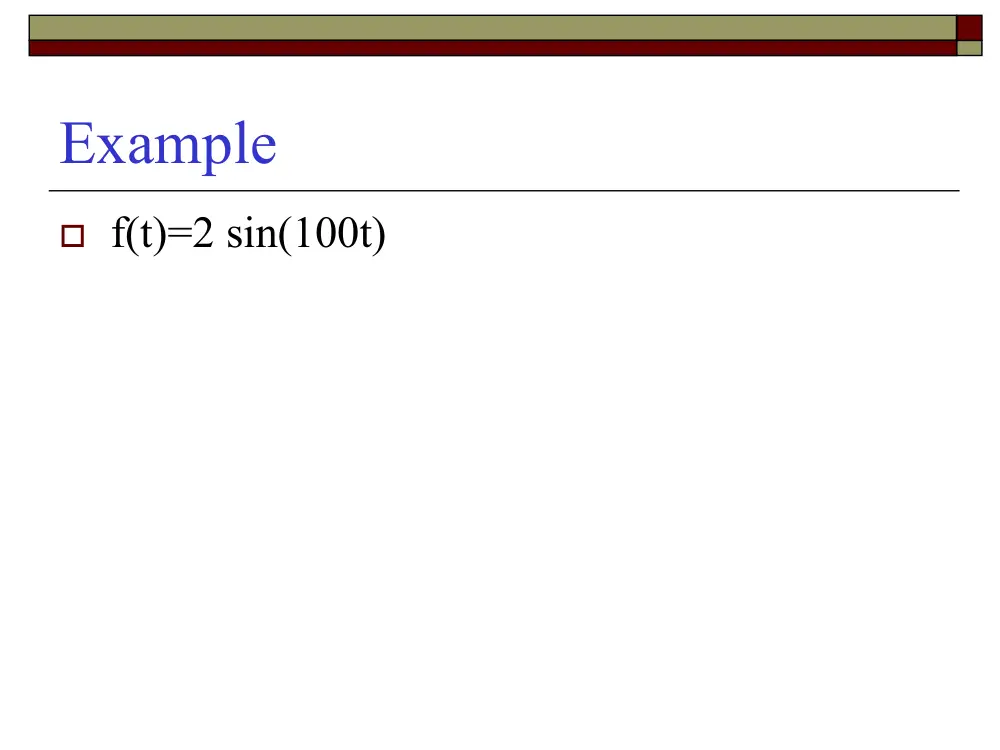Last equation illustrates the fact that the power in a periodic function is distributed over discrete frequencies that are harmonically related to one another ⇒ ⎪⎩ ⎪⎨ ⎧ = ≠ = ∫ − − ω m n T m n 0 dt e / 2 T / 2 T t (j n m) 0 ∑ ∫ ∑ ∞ =−∞ − ∞ =−∞ = ⇒ = = n 2 n 2 / 2 T T / 2 n 2 n F dt )t( f T 1 P F T T P Example � f(t)=2 sin(100t) The Fourier Transform Given a non-periodic (Aperiodic) signal f(t), the Fourier transform of f(t), if it exists, is given by: dt e)t( f t( )} FT f{ F( ) j t ∫ ∞ ∞ − − ω = ω = The Fourier Transform Pairs df F f( e) )t( d or f e) F( 2 1 )t( f dt e)t( f ( ) F ft 2j t j t j π ∞ ∞ − ω ∞ ∞ − − ω ∞ ∞ − ∫ ∫ ∫ = ω ω π = ω = Example 0 a u )t( e )t( f at > = − t f t e atu t ( ) ( ) = − 1 Example f(t)=A rect (t/T) Answer: f t( ) t T/2 A −T/2 ATSa ( T / 2) AT sin( T / 2) 2 T 2A sin F( ) = ω ω ⎟ = ⎠ ⎞ ⎜ ⎝ ⎛ω ω = ω (ωT / 2) The Sa function ATSi ( T ) ω 2 ω AT Existence of The Fourier Transform 1. f(t) has a finite number of maxima and minima in any finite time interval 2. f(t) has only a finite number of discontinuities in any finite time interval. 3. f(t) is absolutely integrable Parseval's Theorem for Energy Signals The energy delivered to 1 Ohm resistor by an energy signal f(t) is given by where ∫ ∫ ∞ ∞ − ∞ −∞ = = )t( dt f)t( f dt )t( f E * 2 ∫ ∫ ∞ ∞ − ω − ∞ ∞ − ω ω ω π = ω ω π = d e) F ( 2 1 )t( f d e) F( 2 1 )t( f j t * * j t Parseval's Theorem for Energy Signals � Replacing the results of f*(t) into the energy equation, we obtain ∫ ∫ ∞ ∞ − ∞ ∞ − − ⎥ ⎦ ⎤ ⎢ ⎣ ⎡ = dt d e F f t E j t ω ω π ω ( ) ( ) 2 1 * ω ω π ω dt d f t e F j t ∫ ∫ ∞ ∞ − ∞ ∞ − − ⎥ ⎦ ⎤ ⎢ ⎣ ⎡ = ( ) ( ) 2 1 * ∫ ∫ ∞ + ∞ − ∞ −∞ = = ω ω π ω ω ω π d F d F F 2 * ( ) 2 1 ( ) ( ) 2 1 Parseval's Theorem for Energy Signals � Therefore, we can conclude ∫ ∫ ∞ ∞ − ∞ −∞ ω = ω π = dt )t( f F( ) d 2 1 E 2 2 Example: The impulse signal δ(t) 1 e dt e)t( t( )} .FT{ t 0 j t j t = = δ = δ = − ω ∞ ∞ − − ω ∫ Example: Complex Exponential t je t f 0 ( ) ω = ∫ ∞ −∞ − = − ω ω δ ω π ω δ ω e ω d I F T ) j t ( 2 1 )} . { ( . 0 0 } . { 2 1 )} . { ( . 0 0 t je F T I F T ω π ω δ ω = − } . { 2 1 ) ( 0 0 t je F T ω π ω δ ω = − ) ( 2 } { . 0 0 ω πδ ω ω − = t je F T Example: Complex Exponential � From Previous example � We can conclude � Moreover, for ω0=0 ) ( 2 } { . 0 0 ω πδ ω ω − = t je T F ) ( 2 } .FT{e 0 t j 0 πδ ω+ ω = ω − ( ) 2 .FT{1} = πδ ω Example: The sinusoidal functions )] ( ) [ ( 2 e .FT 1 2 e .FT 1 2 e 1 2 e .FT 1 }t T{cos .F 0 0 t j t j t j t j 0 0 0 0 0 + δ ω + ω π δ ω − ω = ⎟ ⎠ ⎞ ⎜ ⎝ ⎛ ⎟ + ⎠ ⎞ ⎜ ⎝ ⎛ = ⎟ ⎠ ⎞ ⎜ ⎝ ⎛ + = ω − ω ω − ω ω [ ]) ( ) ( } {sin . 0 0 0 ω δ ω ω π δ ω ω + − − t = j F T The signum function � The signum function f(t)=sign(t) is defined as: ⎪⎭ ⎪⎬ ⎫ ⎪⎩ ⎪⎨ ⎧ < − = > = 0 T 1 0 t 0 0 t 1 )t( f t sgn( )t 1 −1 Properties of the signum function t sgn( )t 1 −1 � 1.Average value=0 � 2.Piece-wise continuous � 3.Not absolutely integrable. Fourier Transform of sign(t) Since sign(t) is not absolutely integrable, the following approach is used. Let The Fourier transform of g(t) is given by: Therefore, the Fourier transform of f(t)=sign(t) is simply obtained by taking the limit of the Fourier transform of g(t) as a goes to zero. sign )t( e )t( g −a t = + ω ω + = + = − = ∫ ∫ ∫ ∞ + ω − ∞ − − ω ∞ ∞ − − ω − j a 1 a - j -1 dt e dt e dt sgn e.t e T{g t( )} .F 0 t) (a j 0 t) (a j j t t a = jω 2 t( )} F.T{sign Example: The Unit-Step function u(t) 2 sgn( )t 1 2 1 u )t( + = ω = πδ ω + ω πδ ω + = + = ⎟ ⎠ ⎞ ⎜ ⎝ ⎛ ⎟ + ⎠ ⎞ ⎜ ⎝ ⎛ = j 1 ( ) j 2 2 1 ( ) 2 2 1 2 .FT{sgn(t)} 1 2 .FT{1} 1 2 sign )t( .FT 1 2 .FT 1 .FT{u t( )} The FT of a Periodic Function � Let f(t) be a periodic function of frequency ω0. The function f(t) can be written using the complex Fourier representation as: � The Fourier transform of f(t) is: ∑ ∞ −∞ = ω = n t jn n 0 F e )t( f ) n F ( 2 dt e F dt e F e t( )} T f{ .F 0 n n n 0 t) (j n n n j t jn 0t n δ ω− ω = π = = ∑ ∫ ∑ ∫ ∑ ∞ −∞ = ∞ ∞ − − ω− ω ∞ −∞ = ∞ ∞ − ∞ −∞ = − ω ω The FT of a Periodic Function ω F( ) ω 2 ω0 ω0 − ω0 − 2 0 ω 2 1 πf 2 πf0 2 πf1 Properties of the Fourier transform 1. Linearity ( ) a F. a F. ( ) t( )} a f. )t( T{a f. .F F ( ) )t( f F ( ) )t( f 2 2 1 1 2 2 1 1 2 2 1 1 ω ω + ↔ + ω ↔ ω ↔ Properties of the Fourier transform 2. Complex conjugate ) F ( )t( f F( ) )t( f * * −ω = ω ↔ Properties of the Fourier transform 3. Duality ) 2 f ( )t( F F( ) )t( f −ω π ↔ ω ↔ Properties of the Fourier transform 4. Scaling ⎟⎠ ⎞ ⎜⎝ ⎛ ω ↔ ω ↔ a F a 1 (at) f F( ) )t( f Properties of the Fourier transform 5. Time Shifting F( ) e t ) t( f F( ) )t( f 0t j 0 ω ↔ − ω ↔ − ω Example � Determine the FT of g(t) as a function of that of f(t) t g t( ) −T T − A A f t( ) t A T / 2 −T / 2 Properties of the Fourier transform 6. Frequency Shifting (VIP) [ ]) F( ) 2 F( 1 )t )t( cos( f F( ) )t( f 0 0 0 ω + ω + ω − ω ↔ ω ω ↔ B − B 1 F( ) ω ω ω ω 0 −ω0 1 2 / F T f t t . { ( ).cos ω0 } Properties of the Fourier transform 7. Differentiation F( ) )t( f ω ↔ j F( ) dt )t( .FT df ω ⎟ ↔ ω ⎠ ⎞ ⎜ ⎝ ⎛ Example f t( ) t T −T 2T −2T A t df t dt ( ) A T / − A T / T −T −2T d f t dt 2 2 ( ) A T / A T / − A T / − A T / T −T −2T t 2T 2T } e e e T {e A ) F( ) j( ( ) G 2T)} t( T) t( T) t( 2T) t( T { A )t( g j 2T j T j T j 2T 2 ω ω − ω − ω + − − ω = ω = ω + + δ + − δ − − δ − δ = Properties of the Fourier transform 8. Integration F. (0) ( ) j F( ) f ( )d T .F t δ ω ω + π ω = ⎪⎭ ⎪⎬ ⎫ ⎪⎩ ⎪⎨ ⎧ τ τ ∫ −∞ Properties of the Fourier transform 9. Time Convolution h(t) impulse response of the system, x(t) is the input, and y(t) is the output. The input-output relationship is given by: LTI System h t( ) x t( ) y t( ) τ − τ ∫ τ = +∞ −∞ )d t( x( h) y )t( Properties of the Fourier transform ( ) ( ) ( ) h t x t y t ∗ = X( )H( ) Y( ) ω ω ω =