EECE 340 Chapter 6, Fall 2011

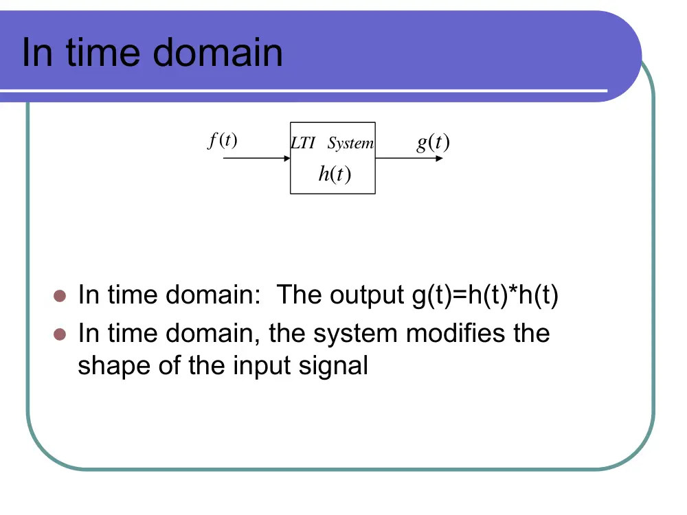
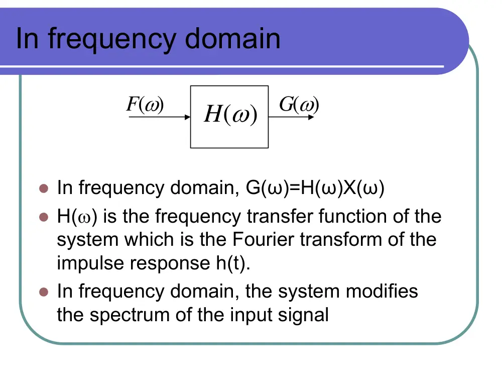
Chapter 6 Filter Characteristics of LTI Systems Contents � In This chapter - Filter characteristics - Bandwidth - Low pass Filter - Band-pass filter - Ideal Filters � We also give some examples In time domain LTI System h t( ) f t( ) g t( ) � In time domain: The output g(t)=h(t)*h(t) � In time domain, the system modifies the shape of the input signal In frequency domain H( ) ω G( ) ω F( ) ω � In frequency domain, G(ω)=H(ω)X(ω) � H(ω) is the frequency transfer function of the system which is the Fourier transform of the impulse response h(t). 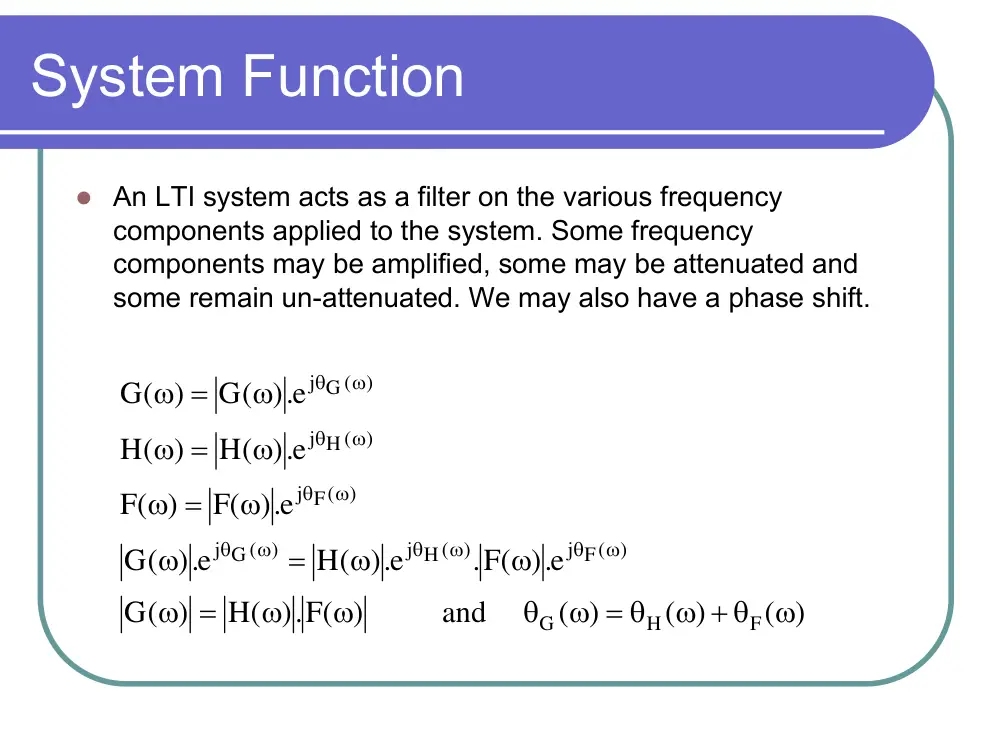� In frequency domain, the system modifies the spectrum of the input signal System Function � An LTI system acts as a filter on the various frequency components applied to the system. Some frequency components may be amplified, some may be attenuated and some remain un-attenuated. We may also have a phase shift. 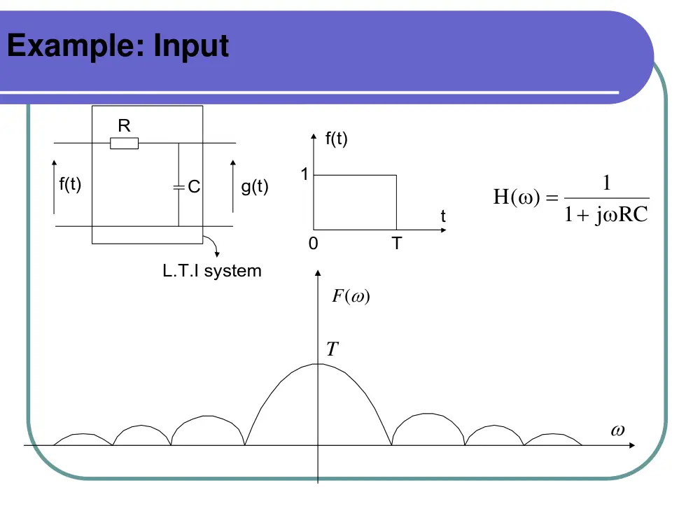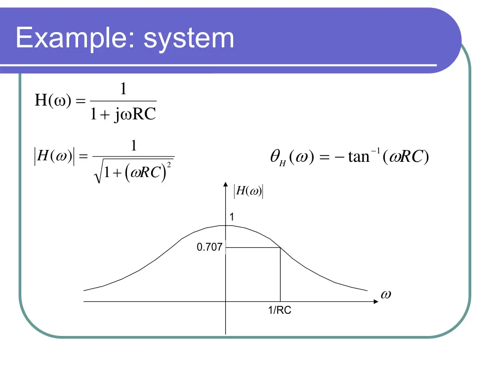( ) ( ) ( ) .) F( ) and H( ( ) G e.) .F( e.) H( e.) ( G e.) F( ( ) F e.) H( ( ) H e.) G( ( ) G F H G j F( ) j H ( ) G ( ) j F( ) j H ( ) j G ( ) j ω ω + θ ω = θ θ ω ω = ω ω ω = ω ω = ω ω = ω ω = ω ω θ ω θ ω θ ω θ ω θ ω θ Example: Input R C f(t) g(t) L.T.I system f(t) t T 1 0 j RC 1 1 H( ) + ω = ω F( ) ω ω T Example: system j RC 1 1 H( ) + ω = ω ( ) H RC ( ) ω ω = + 1 1 2 θ ω ω H RC ( ) tan ( ) = − −1 H( ) ω ω 1 1/RC 0.707 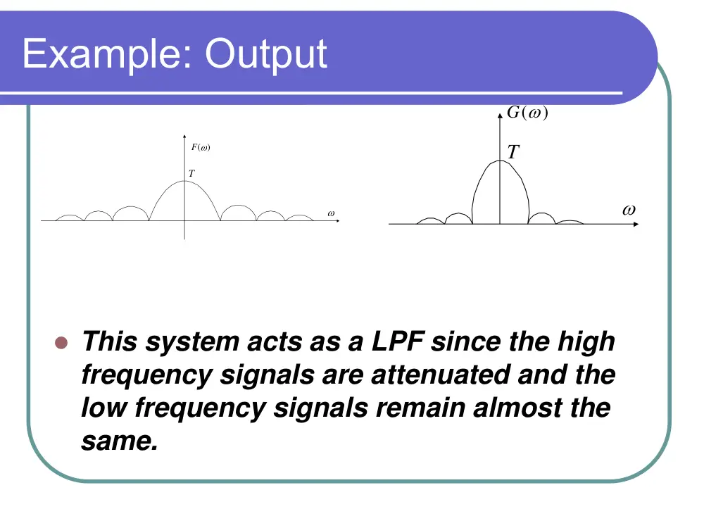Example: Output � This system acts as a LPF since the high frequency signals are attenuated and the low frequency signals remain almost the same. F( ) ω ω T G( ) ω ω T Bandwidth � Bandwidth is a measure of frequency range in Hertz, of a signal or system. � Communication signal bandwidth is the (positive) range of frequencies occupied by a modulated carrier wave � Only the positive frequency plane is counted. Do not count the symmetric negative frequency plane. 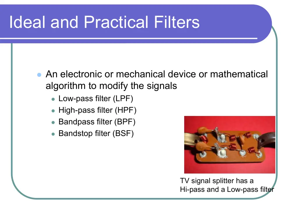� If considering the frequency range where a signal’s FT is non-zero, then many practical systems occupies infinite bandwidth � this is no good Ideal and Practical Filters � An electronic or mechanical device or mathematical algorithm to modify the signals � Low-pass filter (LPF) � High-pass filter (HPF) � Bandpass filter (BPF) � Bandstop filter (BSF) TV signal splitter has a Hi-pass and a Low-pass filter Gain of the filter � The gain of the system is denoted by α(ω)=|H(ω)|. The decibels unit is usually used for the gain H( ) 20.log ) ( 10 ω α′ ω = Bandwidth of a Low Pass Filter The bandwidth of a LP system is defined as the positive frequency components at which the amplitude response |H(ω)| is 1/√2 times the value at zero frequency or the frequency at which the gain drops by 3 dB below its value at zero frequency. Example H( ) ω ω A/ 2 A W BW 20 0 20 0 2 20 0 20 0 20 2 3 0 10 10 10 10 10 .log ( ) .log ( ) ? .log ( ) .log ( ) .log ( ) H H db H H db where H A − = ⇒ − − ≈ = Spectrum of a Voice signal Bandwidth of a band-pass system (filter) � For a band-pass system (filter), the bandwidth is defined as the range of positive frequencies over which the amplitude response |H(ω)|remains within 1/√2 times its value at the mid- band frequency � ωu=upper frequency, ωM=middle frequency, and ωL=Lower frequency ωM − ω M H( ) ω ω ωU ω L −ωL −ωU 1 2 / 1 Bandwidth U L = ω − ω � Ideal low-pass filter � Magnitude response has ideal (sharp) stopband, has ideal bandwidth f0 . � Every frequency lower than f0 can pass, others can not. � Phase response can have linear phase response or non-linear phase response � The non-ideal (practical) filter response may look like (f) −f0 f0 0 |H(f)| f f θ (f) −f0 f0 0 |H(f)| f f θ Ideal filter is a very useful tool for analyzing communication systems. Ideal Band-pass filter � An ideal filter passes without distortion all frequency components between its lower frequency and its upper frequency. Outside this range, the ideal filter is assumed to have zero magnitude 2 f |H(f)| 0 f1 f2 −f1 −f Impulse response of an ideal low-pass filter: As h(t)#0 for t<0 Therefore the ideal low-pass filter is not a causal system. ⎭ ⎬ ⎫ ⎩ ⎨ ⎧ < ω < − ω = − ω θ ⎭ ⎬ ⎫ ⎩ ⎨ ⎧ < ω < − = ω ω = ω ω θ Otherwise 0 W W t. ( ) and Otherwise 0 W W 1 ( ) H e.) H( ( ) H 0 H H ( ) j t)] W Sa [W t( )t( h 0 − π = h t( ) t W/π t0 Impulse Response of a band-pass filter � Left for you to do Example: Determine the spectrum of y(t). y t( ) sinω0t r t 1( ) r t 2( ) r t 3( ) r t 4( ) r t 5( ) r t 6( ) cosω0t sinω1t cosω1t x t( ) BPF BW W @ω0 2 = BPF BW W @ω0 2 = X( ) ω ω W −W 1 × × × × × Example: Determine the spectrum of z(t) H1( ) ω H2( ) ω H1( ) ω H2( ) ω cos120πt cos120πt x t( ) y t( ) × × ∑ ∑ z t( ) 1 2 3 4 5 6 5π −5π 115π 120π 125π X( ) ω −125π −120π −115π Given H1( ) ω ω ω H2( ) ω 115π 120π 125π −120π 5π − 5π 1 1