EECE 340 Chapter 7, Fall 2011

Chapter 7 Application of the Fourier Transform Amplitude Modulation Overview of Continuous Modulation � The purpose of a communication system is to transmit information-bearing signals or base-band signals through a communication channel separating the transmitter from the receiver. � The term base-band is used to designate the band of frequencies representing the message signal. � The voice signal has a maximum frequency component of 3.3 KHz where the carrier frequency ƒc is 540<ƒc<1600 KHz � A shift of the range of frequencies in a signal is accomplished by using modulation which is defined as the process by which some characteristic of the carrier is varied in accordance with a modulating wave. Overview of Continuous Modulation � Modulating signal: another name for the message signal, or the signal to be modulated � Modulated signal: the signal to be transmitted, or the signal obtained after modulation What is modulation? 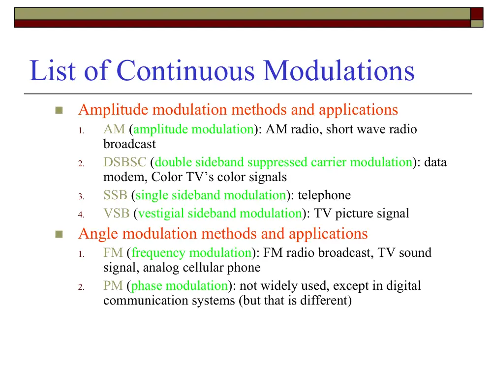� Change baseband signal into passband signal (shift frequency of message signal from low to high) � Change some characteristics of a carrier according to a message signal � Add the message information into the carrier φ( )t List of Continuous Modulations � Amplitude modulation methods and applications 1. AM (amplitude modulation): AM radio, short wave radio broadcast 2. DSBSC (double sideband suppressed carrier modulation): data modem, Color TV’s color signals 3. SSB (single sideband modulation): telephone 4. VSB (vestigial sideband modulation): TV picture signal � Angle modulation methods and applications 1. FM (frequency modulation): FM radio broadcast, TV sound signal, analog cellular phone 2. 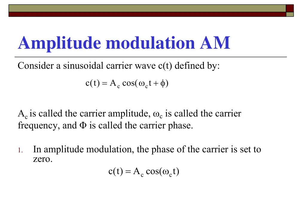PM (phase modulation): not widely used, except in digital communication systems (but that is different) Amplitude modulation AM Consider a sinusoidal carrier wave c(t) defined by: Ac is called the carrier amplitude, ωc is called the carrier frequency, and Φ is called the carrier phase. 1. In amplitude modulation, the phase of the carrier is set to zero. 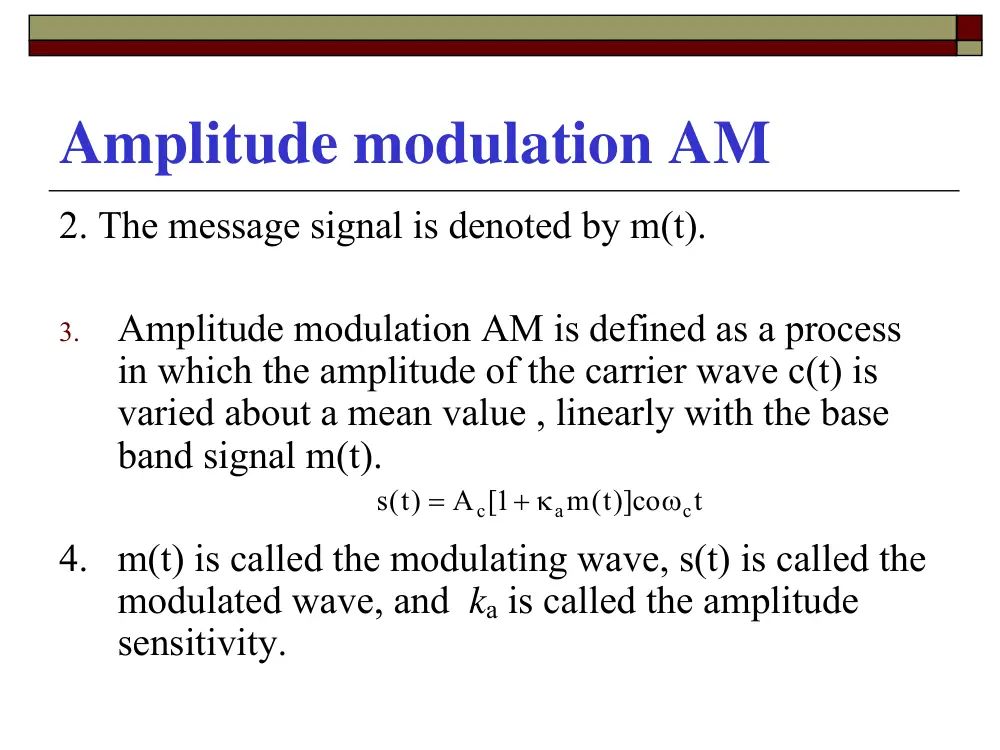) t A cos( )t( c c c + φ ω = )t A cos( )t(c c c ω = Amplitude modulation AM 2. The message signal is denoted by m(t). 3. Amplitude modulation AM is defined as a process in which the amplitude of the carrier wave c(t) is varied about a mean value , linearly with the base band signal m(t). 4. m(t) is called the modulating wave, s(t) is called the modulated wave, and ka is called the amplitude sensitivity. 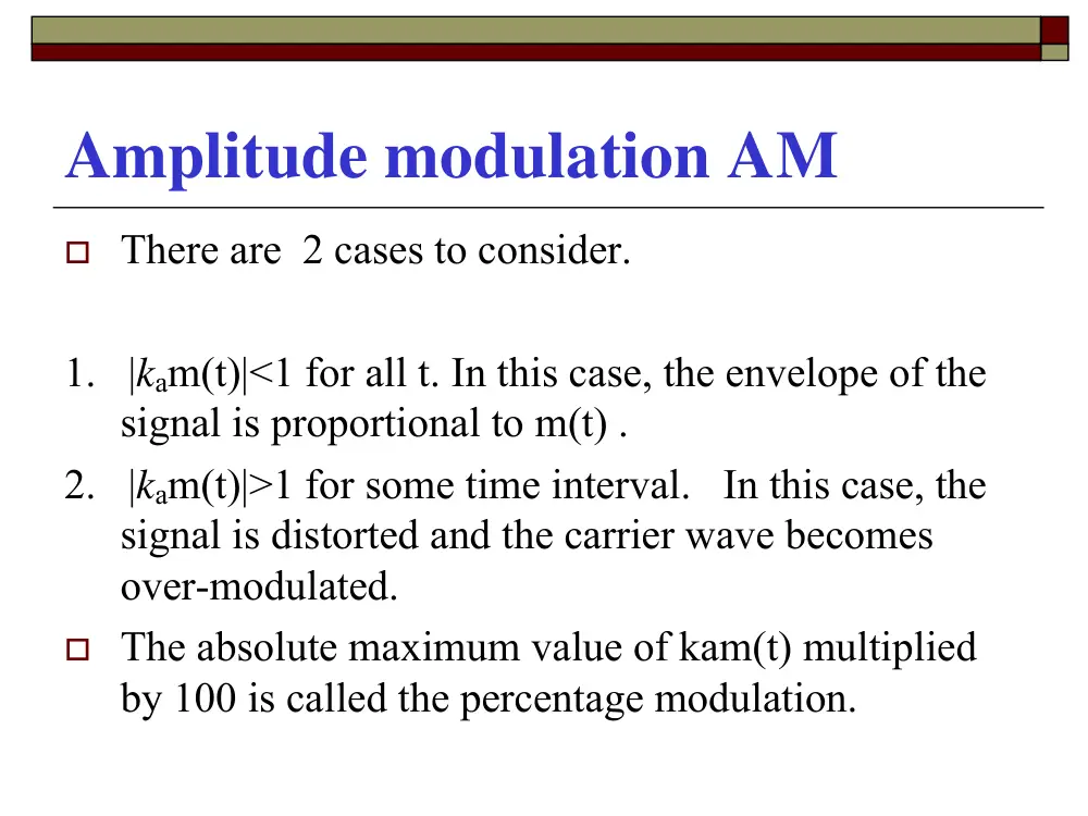t m t( )]co A 1[ )t(s c a c ω + κ = Amplitude modulation AM � There are 2 cases to consider. 1. |kam(t)|<1 for all t. In this case, the envelope of the signal is proportional to m(t) . 2. |kam(t)|>1 for some time interval. In this case, the signal is distorted and the carrier wave becomes over-modulated. � The absolute maximum value of kam(t) multiplied by 100 is called the percentage modulation. 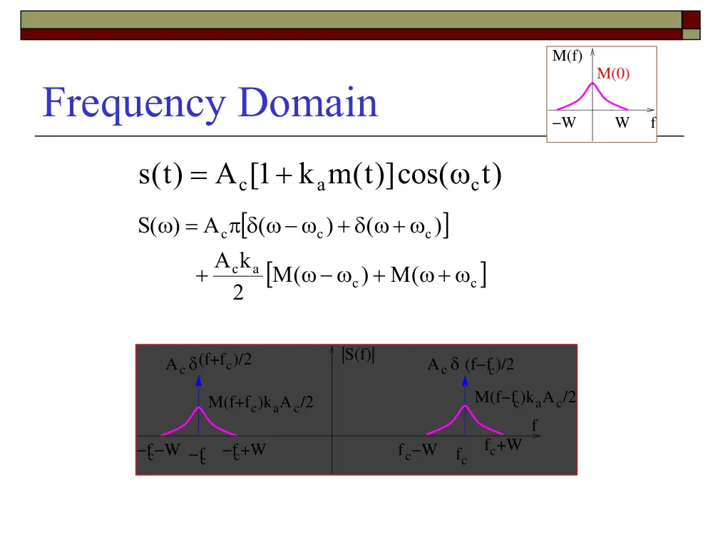� Compare carrier frequencies, and over-modulation f M(f) M(0) W −W Frequency Domain )t k m t( )]cos( A 1[ )t(s c a c ω + = [ ] [ c ] c a c c c c M( ) M( 2 A k ) ( ) ( A ( ) S ω+ ω + ω− ω + + δ ω+ ω π δ ω− ω = ω /2 f |S(f)| δ(f+fc)/2 M(f+fc)kaAc/2 −fc −fc+W −fc−W fc fc+W fc−W Ac Ac δ (f−fc)/2 M(f−fc)kaAc f M(f) M(0) W −W Observations /2 f |S(f)| δ(f+fc)/2 M(f+fc)kaAc/2 −fc −fc+W −fc−W fc fc+W fc−W Ac Ac δ (f−fc)/2 M(f−fc)kaAc � The bandwidth of the AM signal is 2W (twice the bandwidth of the message signal) � For positive frequencies, the portion of the spectrum of an AM wave lying above is called upper sideband (USB) . The other portion is the lower sideband (LSB). � Large Carrier (to be shown later) � Or this reason, it is also called Double Side-Band Large Carrier (DSBLC) Example: Single-tone modulation � In this case, we assume that m(t)=amcos(ωmt) � The corresponding AM wave is given by: � Let kaam=µ<1 be the modulation factor )t t)]cos( cos( k a A 1[ )t(s c m m a c ω ω + = )t t)]cos( cos( A 1[ )t(s c m c ω ω + µ = Example: Single-tone modulation )t t)]cos( cos( A 1[ )t(s c m c ω ω + µ = � Let Amax denotes the maximum value of the envelope of s(t) � Let Amin denotes the minimum value of the envelope of s(t) � From the above equation, Amax = Ac [1+µ] and Amin = Ac [1-µ]. That is : � µ is also called the modulation index of the waveform. min max min max A A A A + − µ = Example: Single-tone modulation Frequency Domain )t t)]cos( cos( A 1[ )t(s c m c ω ω + µ = )t )t cos( cos( A )t A cos( )t(s c m c c c ω ω µ + ω = t) 2 cos( A )t 2 cos( A )t A cos( )t(s m c c m c c c c ω − ω µ + ω + ω µ + ω = [ ] ⎥⎦ ⎤ ⎢⎣ ⎡ + δ ω+ ω − ω δ ω− ω + ω + + δ ω+ ω + ω µ δ ω− ω − ω + + δ ω+ ω π δ ω− ω = ω m c m c m c m c c c c c ( ) ( ) ( ) ( 4 A ) ( ) ( A ( ) S The transmission bandwidth is: 2ωm rad/s m ω rad/s Carrier and sideband power in AM � By definition, the average power of s(t) across 1Ω Resistor is given by: Carrier Upper sideband Lower Sideband power power power )t t)]cos( cos( A 1[ )t(s c m c ω ω + µ = t) 2 cos( A )t 2 cos( A )t A cos( )t(s m c c m c c c c ω − ω µ + ω + ω µ + ω = 2 2 A 2 2 A 2 (A ) P 2 c 2 c c 2 ⎟⎠ ⎞ ⎜⎝ ⎛ µ ⎟⎠ + ⎞ ⎜⎝ ⎛ µ + = Power ratio � An important measure in AM is the ratio of sideband power to the total power. For a single-tone modulation, this ratio, X, is given by: � X is dependent only on the modulation factor µ 2 . 2 1 2 A 4 1 2 A A 4 1 X 2 2 2 2 c 2 2 2 c 2 c 2 + µ µ = µ + µ = µ + µ = Power ratio . 2 X 2 2 µ + µ = � For the case where µ=1, X=1/3; that is, if 100% modulation is used, the total power in the 2-sidebands is only 1/3 (one-third) of the total power in the modulation wave. 67% of the power is expanded in the carrier and represents wasted power as far as the transfer of information is concerned Envelope detector � An envelope detector is a circuit that produces an output signal that follows the envelope of the signal waveform exactly. � The simplest form is a nonlinear circuit with a fast charge time and slow discharge time. How does it work? � During the positive half cycle of the input signal, the capacitor charges to the peak value of v1(t) = v2(t). � When v1(t) < v2(t), the diode is turned off. The capacitor discharges through the resistor to the next peak value when v1(t) becomes greater than the capacitor voltage. The discharging time : τ = RC . � RC should be adjusted, as the maximum negative rate of the envelope will never exceed the exponential discharge rate. � A low-pass filter is then used to eliminate the unwanted harmonic content. � Note that the envelope detector is simple, efficient, and cheap to built. � Example 1 � For the AM signal spectrum pictured in the figure below, calculate � The message signal frequency fm � The magnitude of the upper sideband � The bandwidth � Percentage modulation f(kHz) |S(f)| 20 5 5 20 5 5 810 813 � Example 2 � A single-tone modulated signal is shown below. The envelope has maxima 18 and minima 2. � What is the carrier amplitude Ac? � What is the percentage modulation? t 18 2 � Example 3 � An AM modulation with carrier frequency fc=540 kHz, carrier amplitude Ac=20. Message signal is single tone with fm=10kHz, whose amplitude Am can make the carrier amplitude changing +/-7.5 around Ac=20. � What is percentage modulation? � Find the modulated signal. Simple AM Modulator Major Properties of AM � Advantages � Simplicity in implementation, especially the receiver � The major reason that AM was the first & most popular broadcasting methods during early days � Disadvantages � Waste power and bandwidth � Carrier components wastes a major portion power, but carrier does not have message information � Both USB and LSB are transmitted, which carry the same message information Ways for improvement � To enhance power efficiency � Reduce/remove carrier: DSB-SC � Remove one/partial sideband: SSB, VSB � To enhance bandwidth efficiency � Remove one/partial sideband: SSB, VSB � Multiplex two message signals together: QAM � Cost for the improvement � More expensive implementation � The simple envelope detector is no longer applicable History of AM radio � First AM radio broadcast experiment: 1906, by Reginald Fessenden � First commercial AM radio service: 1920, KDKA in Pittsburgh, PA. � 1020 kHz carrier, 50 KWatts. � There are 16265 AM stations worldwide � DSB-SC modulated signal waveform ( ) ( )cos(2 ) c c s t A m t π f t = π m(t) s(t) Accos(2 fct) m(t) t phase reversals s(t) t Double Sideband Suppressed Carrier (DSB-SC) Signal Spectrum 1. The Transmission bandwidth: 2W 2. Transmission power = Upper sideband power + Lower sideband power [ ]) M( ) 2 M( A S( ) c c c ω+ ω + ω− ω = ω M(f) W −W f 2W f |S(f)| M(f+fc) −fc −fc+W −fc−W fc fc+W fc−W M(f−fc) A /2 c Ac /2 2W DSB Modulator, Modulator � Block diagram of DSB modulator � Mixer: a nonlinear device (such as multiplier) that accepts two inputs, the sum or difference of their frequency is in the outputs ( ) ( )cos(2 ) c c s t A m t π f t = We may remove bandpass filter. s(t) m(t) Accos(2 fct) π Filter Bandpass Demodulation of DSB-SC wave Coherent detector � A method of demodulating DSBSC known as coherent detection or synchronous detection is based on multiplying (shifting) the received signal with a locally generated sine wave and then low-pass filtering the product. It is assumed the local oscillator is exactly coherent or synchronized in both frequency and phase with the carrier wave C(t). Product Modulator Low-pass Filter v0(t) ′ + + A f t ft c c cos[ ] 2 2 π π ∆ Φ s(t) v(t) Local Oscillator [ + ∆ω + ∆φ] ω ω = t t )t cos cos( A m )t( )t( v c c c 2 cases to consider 1. ∆ω=0. In this case, If ∆Φ varies in a random manner, the obtained signal is unacceptable. (In practice) 2. ∆Φ=0. In this case, Undesirable and unacceptable distortion Therefore, circuitry must be provided in the receiver to maintain the local oscillator in perfect synchronization in both frequency and phase, with the carrier wave used to generate DSBSC wave in the transmitter. The resulting receiver complexity is the price that must be paid for suppressing the carrier wave to save transmitter power ) cos( 2 m )t( A )t( v c o ∆φ = )t cos( 2 m )t( A )t( v c o ∆ω = The Hilbert Transform David Hilbert 1862-1943 German Math Norbert Wiener (1894-1964). Mathematician, MIT Professor. Introduced HT into communications. The Hilbert Transform Consider a signal g(t) whose Fourier transform G(ω). The Hilbert transform of g(t), denoted by , is defined as: )t( gˆ �( ) ( ) g t g t d = − −∞ ∞ ∫ 1 π τ τ τ g(t) h(t)= πt 1 g(t) Facts about Hilbert Transform In Frequency Domain � The Fourier transform of the signal 1/πt is given by: � where ⎭⎬⎫ ⎩⎨⎧ π ω ⋅ ω t 1 ) = G( ) FT ( Gˆ ∫ ∞ ∞ − − ω ω = − π ⎭⎬⎫ = ⎩⎨⎧ π jsgn( ) dt t e 1 t 1 FT t j ⎪⎭ ⎪⎬ ⎫ ⎪⎩ ⎪⎨ ⎧ ω < − = ω > ω = ω 0 1 0 0 0 1 sgn( ) In Frequency Domain ⎪⎭ ⎪⎬ ⎫ ⎪⎩ ⎪⎨ ⎧ ω < = = ω ω > = − ω = = − ω π π − 0 e j 0 0 0 e j jsgn( ) ( ) H / 2 j / 2 j This device (as shown in the right figure) produces a -90° phase shift for all positive frequencies and a 90° phase shift for all negative frequencies Examples 1. What is the Hilbert transform of 1? 2. Find the Hilbert transform of g(t)=Acos(ωct)? 3. Find the Hilbert transform of g(t)=Asin(ωct)? Properties of the Hilbert Transform 1. A signal g(t) and its Hilbert transform have the same autocorrelation function 2. A signal g(t) and its Hilbert transform are orthogonal. 3. The Hilbert transform of the Hilbert transform of g(t) = -g(t). Pre-envelope of a signal g(t) Pre-envelope of a signal g(t) Single-Sideband Modulating (SSB) � AM and DSBSC modulation are wasteful of bandwidth because they both require a transmission bandwidth equal to twice the message bandwidth. One half of the BT is occupied by the upper sideband and the other is occupied by the lower sideband. Both USB and LSB are uniquely related to each other by virtue of their symmetry about the carrier frequency. That is if the carrier and one sideband are superposed, no information is lost. � Therefore, the benefits of SSB modulation are reduced bandwidth ( the same as the modulating signal ) and the elimination of the high-power carrier wave. Single-Sideband Modulating (SSB) � The time-domain representation of a SSB wave s(t) is : � The - sign stands for the upper sideband where the + sign stands for the lower sideband. t A m t t A m t s t c c c c ω ω ˆ ( )sin 2 ( )cos 2 ( ) ∓ = Frequency Analysis � How SSB representation was obtained?