EECE 340 Chapter 8, Fall 2011

Chapter 8 Application of the Fourier Transform Frequency Modulation Characteristics of FM � Why need Frequency modulation? � Better noise reduction � Improved system fidelity � Disadvantages � Low bandwidth efficiency � Complex implementations � Applications � FM radio broadcast � TV sound signal � Two-way mobile radio � Cellular radio � Microwave and satellite communications Definition In this modulation, the frequency of the carrier is varied linearly with the base-band signal m(t). Where kf is a constant and called frequency sensitivity. 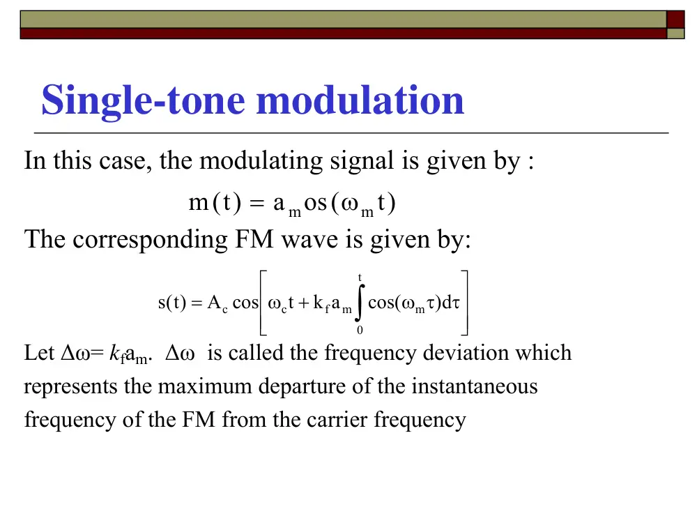The frequency-modulated wave is therefore described in the time- domain by: k m )t( )t( f c i = ω + ω ∫ ∫ τ τ + τ = ω τ = θ t 0 f c t 0 i i m( )d k t f ( )d )t( ⎥ ⎥ ⎦ ⎤ ⎢ ⎢ ⎣ ⎡ τ τ + ω = ∫ t 0 f c c m ( )d k t cos A )t( s Figure of FM modulation Single-tone modulation In this case, the modulating signal is given by : The corresponding FM wave is given by: Let ∆ω= kfam. ∆ω is called the frequency deviation which represents the maximum departure of the instantaneous frequency of the FM from the carrier frequency )t a os( )t( m m m ω = ⎥ ⎥ ⎦ ⎤ ⎢ ⎢ ⎣ ⎡ τ ω τ + ω = ∫ t 0 m m f c c )d cos( k a t A cos )t(s Single-tone modulation With ∆ω= kfam, the FM waveform becomes: The ratio of ∆ω to the modulation frequency is called the modulation index of the FM wave and it is denoted by β The above is the time-representation of an FM wave for single-tone modulation ⎥⎦ ⎤ ⎢⎣ ⎡ ω ω + ∆ω ω = t sin t cos A )t( s m m c c [ ]t sin t A cos )t(s m c c ω +β ω = Types of FM Modulation � Depending on the value of the modulation index β, we may distinguish two cases of frequency modulation: 1. Narrow-band FM (NBFM) for small β, β is small compared to 1 radian. β<0.3 is taken to be sufficient, but as high as 0.5 are used. 2. Wide-band FM (WBFM) when β is large compared to 1 radian Narrow-band Frequency modulation (NBFM) In general, the FM wave is given by: For small β, That is; ]t sin t cos[ A )t( s m c c ω + β ω = t]. sin t sin[ sin A ]t sin t cos[ cos A )t( s m c c m c c ω β ω − ω β ω = t sin ]t sin sin[ 1 ]t sin cos[ m m m ω ≅ β ω β ≅ ω β t tsin sin A t A cos )t(s m c c c c ω ω β − ω = NBFM and AM Note hat the expression representing NBFM wave is similar to that of AM for single-tone modulation t) 2 cos( A t) 2 cos( A t A cos )t( s m c c m c c c c FM ω + ω β + ω − ω β − ω = t) 2 cos( A t) 2 cos( A t A cos )t( s m c c m c c c c AM ω + ω β + ω − ω µ + ω = � Figure Spectrum of the Frequency modulation Spectrum of the Frequency modulation Spectrum of the Frequency modulation Spectrum of the Frequency modulation Properties of the Bessel Function Transmission Bandwidth of FM waves � In theory, FM wave contains an infinite number of side-bands. However, The magnitude of the higher- order side-bands becomes negligible and the power is contained within a finite bandwidth. � A side-band is significant if its magnitude is equal to or exceeds 1 % of the unmodulated carrier; |Jn(β)|>0.01. This number can be obtained from the table for different values of β. Transmission Bandwidth of FM waves Transmission Bandwidth of FM waves Transmission Bandwidth of FM waves β) fc fc+fm fc−fm fc+2fm fc−2fm −fc−fc+fm −fc−fm |S(f)| f J0(β) J0(β) J1(β) J−1(β) J1(β) J−1(β) J2(β) J−2(