EECE 340 Chapter 9, Fall 2011

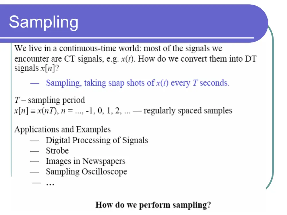
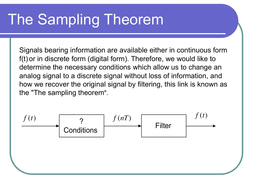
Chapter 9 Sampling Theorem Sampling The Sampling Theorem Signals bearing information are available either in continuous form f(t)or in discrete form (digital form). Therefore, we would like to determine the necessary conditions which allow us to change an analog signal to a discrete signal without loss of information, and how we recover the original signal by filtering, this link is known as the "The sampling theorem". ? 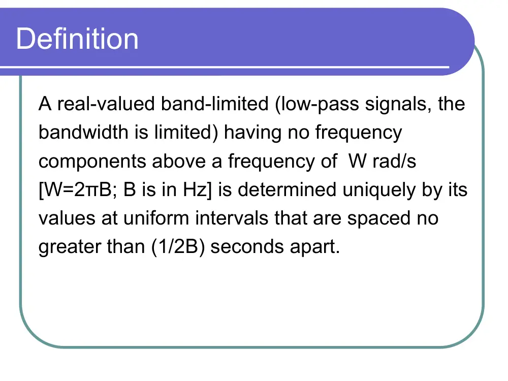Conditions Filter f t( ) f t( ) f nT ( ) Definition A real-valued band-limited (low-pass signals, the bandwidth is limited) having no frequency components above a frequency of W rad/s [W=2πB; B is in Hz] is determined uniquely by its values at uniform intervals that are spaced no greater than (1/2B) seconds apart. 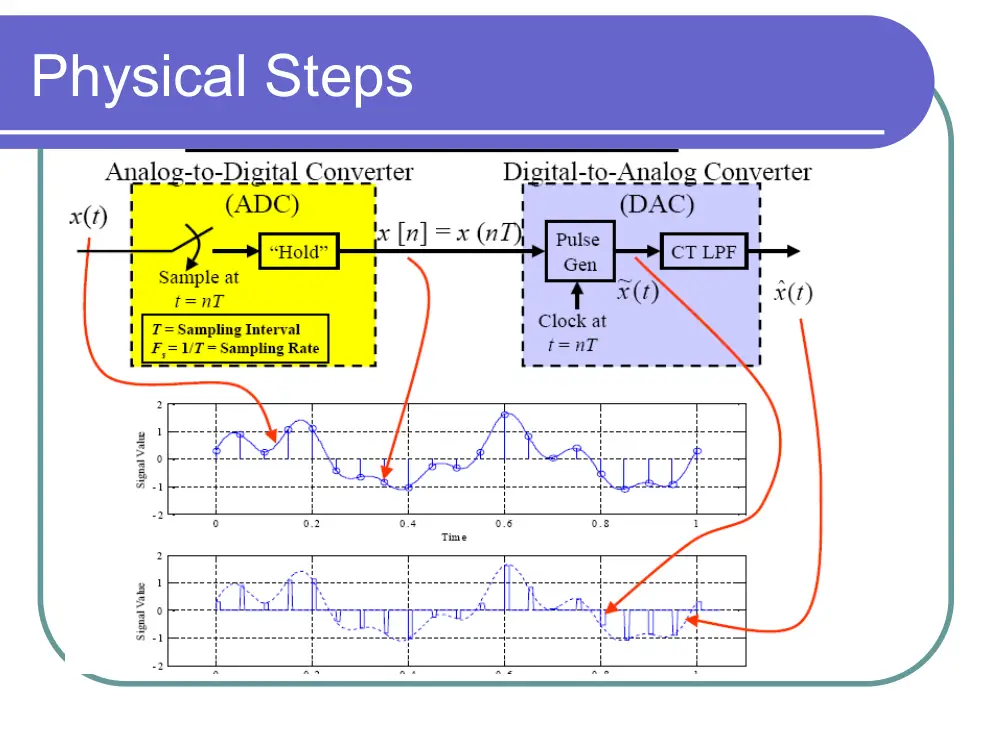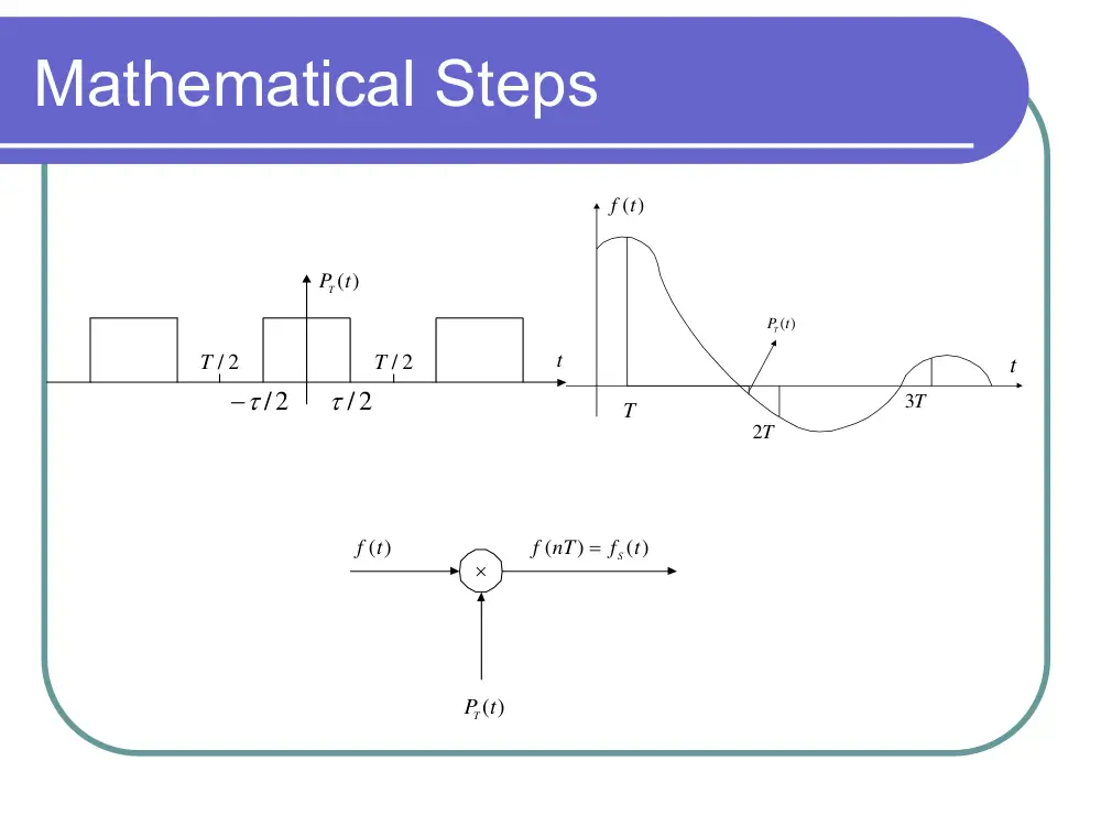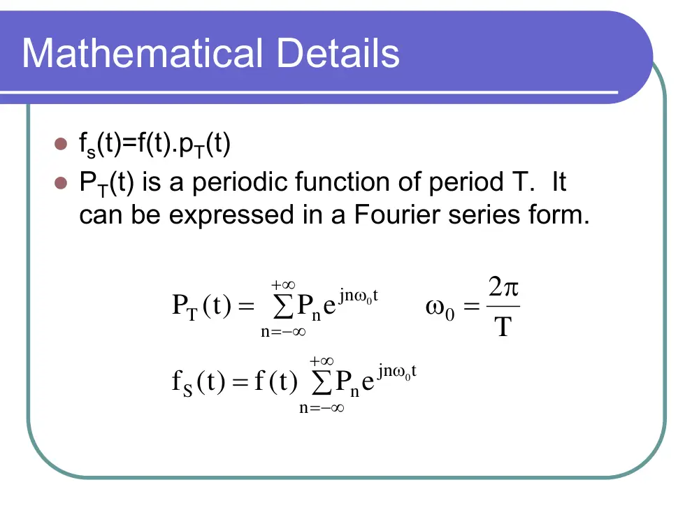Physical Steps Mathematical Steps P t T( ) t τ / 2 −τ /2 T / 2 T / 2 f t( ) P t T( ) 2T T 3T t P t T( ) f t( ) f nT f S t ( ) ( ) = × Mathematical Details � fs(t)=f(t).pT(t) � PT(t) is a periodic function of period T. It can be expressed in a Fourier series form. t jn n n S 0 t jn n n T 0 0 P e )t( f )t( f T 2 P e )t( P ω ∞ + −∞ = ω ∞ + −∞ = ∑ = π ω = = ∑ The Fourier Transform of fs(t) t jn n n S 0 t jn n n T 0 0 P e )t( f )t( f T 2 P e )t( P ω ∞ + −∞ = ω ∞ + −∞ = ∑ = π ω = ∑ = ) n P F( ( ) F e)t( f P ( ) F dt e P e )t( f dt e)t( f ( ) F 0 n n S t) n (j n S t j n t jn n j t S S 0 0 ω − ω = ∑ ω ∫ = ∑ ω ∑ = ∫ = ∫ ω ∞ −∞ = − ω− ω ∞ ∞ − ∞ ∞ − − ω ∞ −∞ = ω ∞ ∞ − − ω ∞ −∞ Case 1: T<1/2B 2W 2W 1 1 2(2 B) 1 1 2B 1 2 2B 1 2 T; T T 2 0 0 0 0 0 0 ⇒ ω > ⇒ ω < π ⇒ ω < < ω π ⇒ < ω = π π ⇒ = ω F( ) ω ω W −W 1 FS( ) ω ω W −W ω 0 −ω0 P0 P1 P−1 P2 2 ω0 −2 0ω P−2 2W 2W 2W 2W 2W Case 1: T<1/2B � 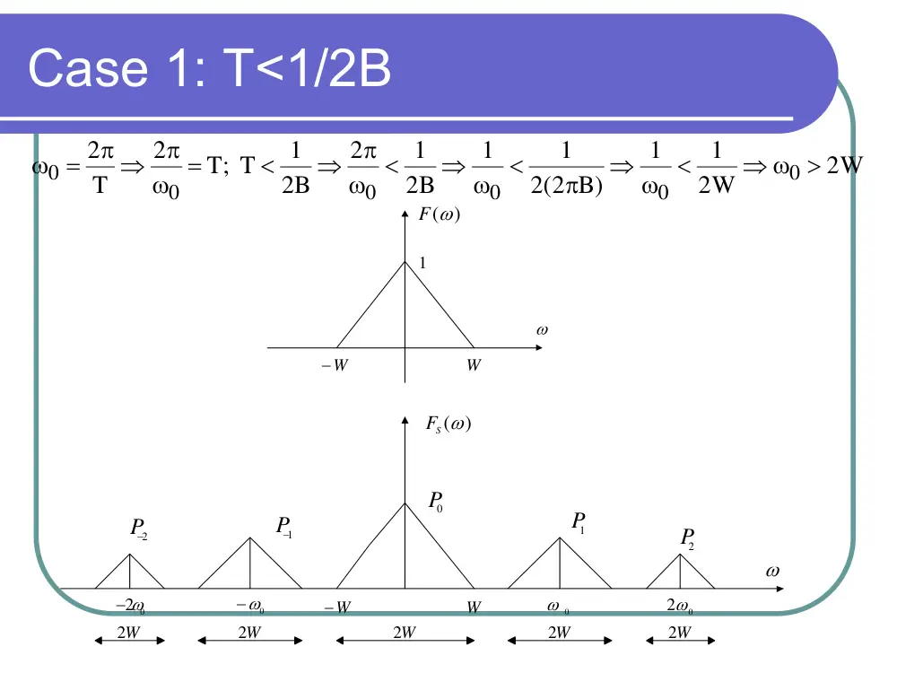Accordingly, the 2-signals would not interfere with each other. The original signal f(t) can be recovered from its sampled version by the use of an LPF of bandwidth W rad/s. � Notation: (1/2B) is called the Nyquist interval , and 1/T is called the Nyquist rate Under sampling Case 2: T>1/2B � In this case, Accordingly, f(t) can not be recovered from its sampled version ω0 < 2W General notes Aliasing: What if the signal f(t) is not band-limited